How to Transpose Data in Excel?

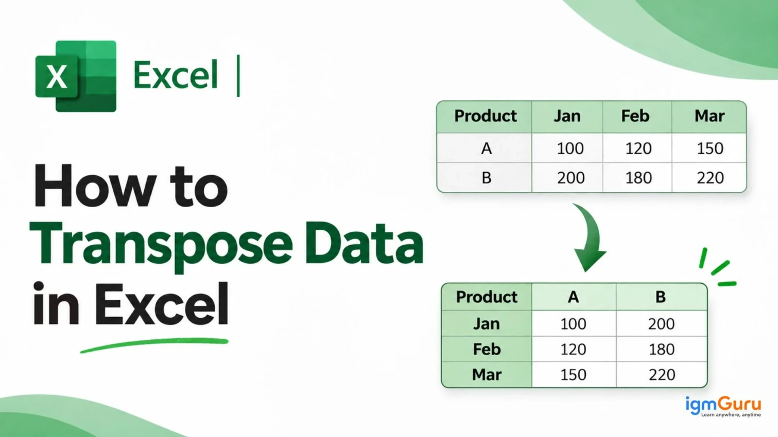
You open a sheet and find the months running down the page. Your report needs them across the top. Retyping everything would take forever and you might make some mistakes.

Excel solves this problem in seconds. In this guide, you will learn how to transpose data in Excel with three reliable methods. You will also see how to handle rows, columns and full tables and how to avoid the most common errors.

Let’s get into it!

In a Nutshell

Excel have several ways from which you can transpose your data, but if you want the quickest way, here it is:

• Select and copy your data (Ctrl + C).
• Right-click on the cell where you want the transposed data to appear
• Select the option “Paste Special"
• Check the "Transpose" box
• Click OK.

I use Excel every day and I am always discovering new ways to make working with data easier. If you are curious, this blog shares a few handy ways to transpose your data that you can explore at your own pace.

Master Advanced Excel. Turn Data Into Insights.

Develop advanced Excel skills in formulas, data analysis, PivotTables, dashboards, and reporting through practical training.

Enroll in Advanced Excel Training →

What Does Transposing Data in Excel Mean?

Transposing in excel simply means when you change your rows to columns and your columns to rows. It rearranges your data by switching its direction while keeping all the original information unchanged.

Transposing data changes its layout by converting rows into columns and columns into rows. The first row becomes the first column, the second row becomes the second column, and the pattern continues for the remaining data.

Here is a small example. This table shows headcount by department:

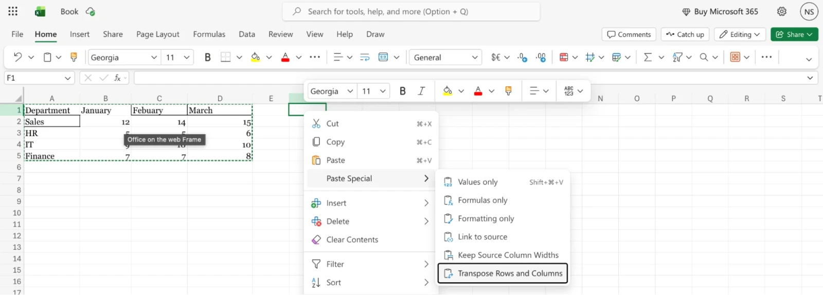
After you transpose it, the departments run across the top and the months run down the side:

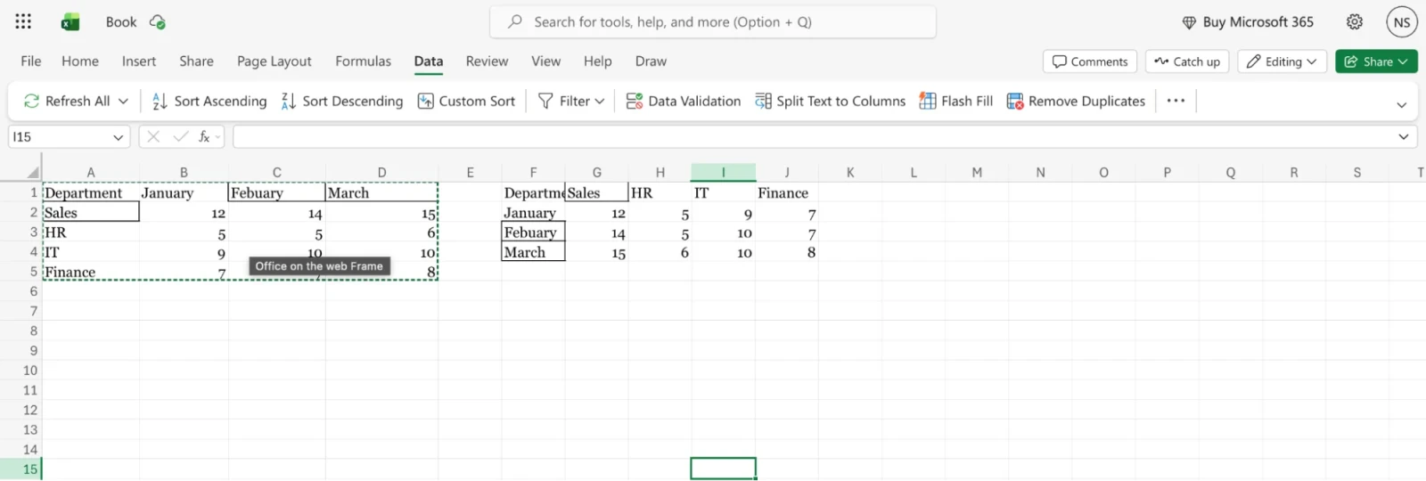
The numbers are the same. Only the direction has changed.

Read Also: Pie Chart in Excel

3 Methods to Switch Rows and Columns in Excel

You can rearrange data in Excel using three different approaches, which mainly depends on your needs and how you want to work with your data.

I will use the same table that I have explained above, placed in cells A1:D5. Each method suits a different situation.

1. Using paste special to transpose data

Paste Special is the fastest way to transpose in Excel. It makes a one-time copy of your data in the new direction.

• Select the data you want to transpose, as in my case the cells are A1:D5.
• Press Ctrl + C to copy it and then click on any empty cell ( such as F1)
• Right click and choose Paste Special.

• In the Paste Special dialog box, tick the Transpose box and click OK.

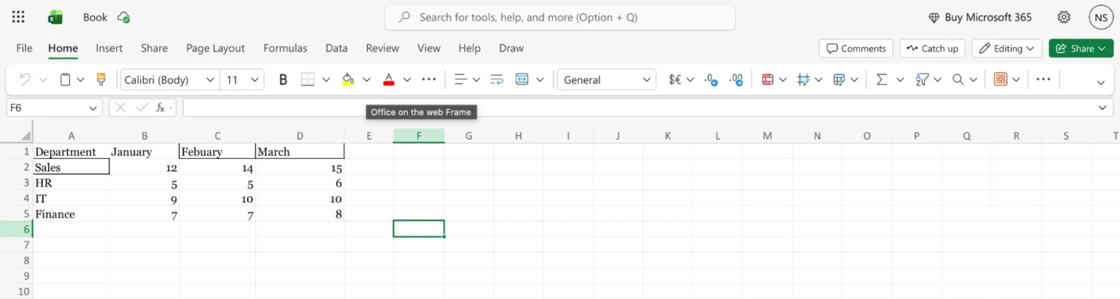
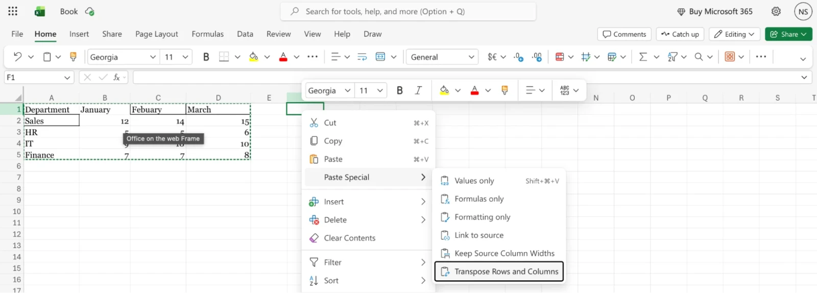
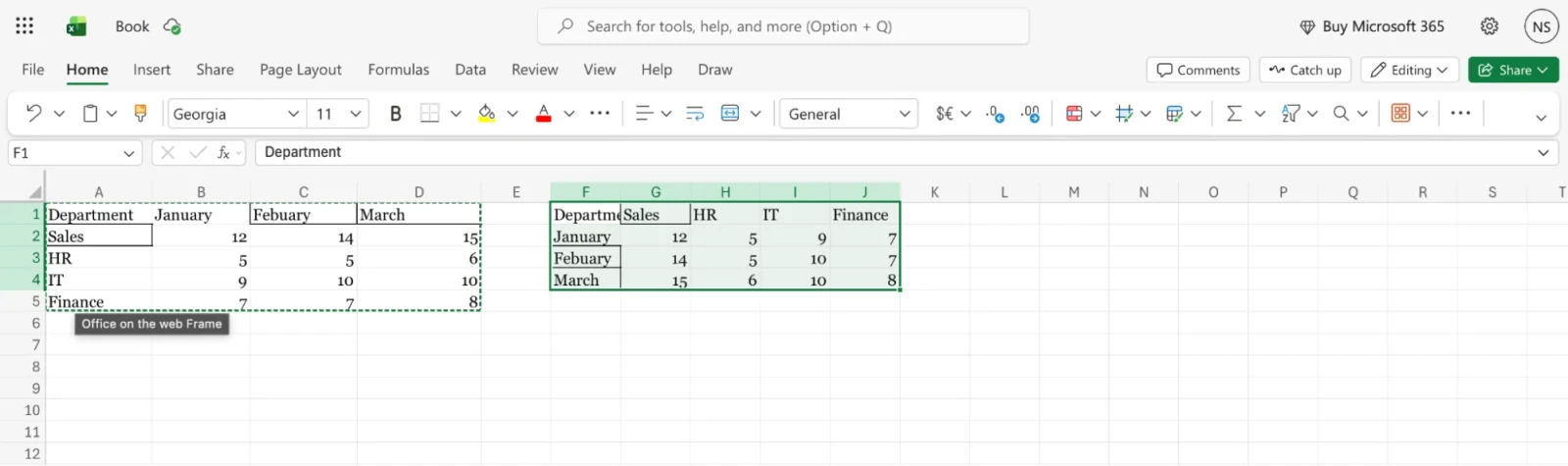
Keyboard shortcut keys: Excel places the flipped table in the new location. You can also use the keyboard. Press Ctrl + Alt + V, then press E and press Enter.

Note: Only use this method when you need a quick fix and your data will not change later.

Advantage: It is simple and it keeps your cell formatting.

Limitation: The result is static. If you edit the source, the transposed copy will not update.

2. Using the TRANSPOSE() function

The TRANSPOSE function in Excel creates a live link to your source. When a source value changes, the transposed value changes too.

The syntax is simple:

The array is the range you want to flip.

In Excel 365, 2021 and 2024:

• Click on any empty cell where you want the transposed data to appear (such as F1).
• Type =TRANSPOSE(A1:D5) to select the data you want to transpose.

• Press Enter to display the transposed data.

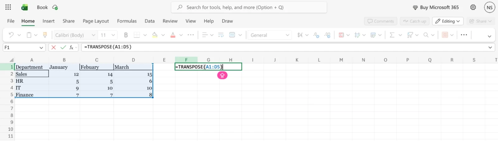
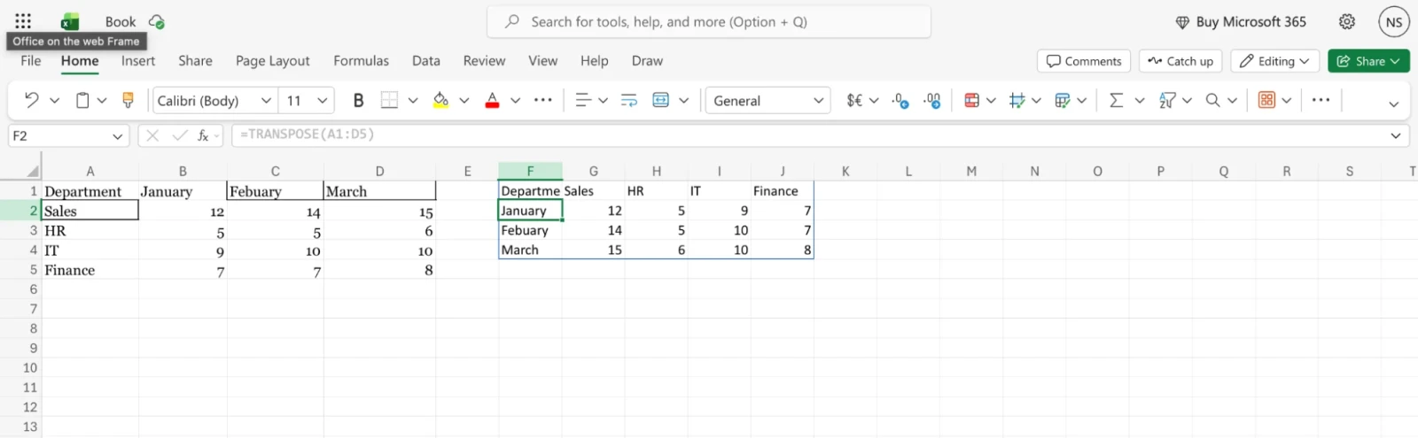
The results spill into the cells around F1 on their own.

In Excel 2019 and earlier:

1. Your source has 5 rows and 4 columns, so select a blank range with 4 rows and 5 columns.
2. Type =TRANSPOSE(A1:D5).
3. Press Ctrl + Shift + Enter.

Excel wraps the formula in curly brackets, which shows it is an array formula.

Note: Only use this method when your source data changes often and you want the new layout to stay current.

Advantage: The result updates automatically.

Limitation: You cannot edit a single cell inside the result. You must also keep enough blank space for the output.

3. Using Power Query to transpose data

Power Query is the best choice for large datasets and repeat work. You build the steps once and refresh them whenever the source changes.

• Click any cell within your data.
• Keep in mind, however, that the versatility of data sources available to Power Query is one of its core advantages.
• Go to the Data tab and select From Table/Range. Click OK if prompted to create a table.
• In the Power Query Editor, click the Transform tab.
• Select Use First Row as Headers, then choose Use Headers as First Row to keep your original headings.
• Click Transpose.
• Select Use First Row as Headers again to set the new headings.
• Go to the Home tab and click Close & Load to bring the transposed data back into Excel.

Excel sends the flipped table to a new sheet. If the source changes later, go to the Data tab and click Refresh All.

Note: Only use this method when you have a large dataset, or you repeat the same cleanup every week or month.

Advantage: You can add more cleanup steps and you can refresh with one click.

Limitation: It takes more steps and it opens a separate editor window.

Also Explore: How to Add a Checkbox in Excel?

How to Rearrange Excel Rows, Columns and Tables

Now we have discussed all those three main methods for transposing your data in excel, let us briefly address some specific scenarios you might face.

How to Transpose Columns to Rows in Excel

Suppose you have monthly sales in B2:B7 and you want them in one row.

• Paste Special: Copy B2:B7, click the first cell of your new row, open Paste Special, tick Transpose and click OK.
• TRANSPOSE function: Type =TRANSPOSE(B2:B7) in the first cell of the new row. In Excel 365, press Enter. In older versions, select a range of 1 row by 6 columns first and then press Ctrl + Shift + Enter.

How to Transpose Rows to Columns in Excel

Now suppose your values sit in B1:G1 and you want them in one column.

• Paste Special: Copy B1:G1, click the first cell of your new column, open Paste Special, tick Transpose and click OK.
• TRANSPOSE function: Type =TRANSPOSE(B1:G1) in the first cell of the new column. In older versions, select a range of 6 rows by 1 column first.

The steps are almost identical in both directions. Excel treats rows and columns as a pair, so one feature handles both jobs.

How to Transpose Tables in Excel

A table has headers, so you need a little more care.

1. Select the full range, including the header row and the label column.
2. Copy it and use Paste Special with Transpose in an empty area.
3. Check that your old headers now sit in the first column and your old labels sit in the first row.

If your data is an official Excel Table (created with Ctrl + T), convert it to a normal range first. You can do this from Table Design by clicking Convert to Range. For very large tables, use Power Query. If you only need part of a table, select just that part before you copy it.

Master Excel Charts. Present Data With Clarity.

Learn to create, customize, and format Excel charts to visualize data and communicate insights effectively.

Enroll in Excel Charts Training →

Important Tips for Transposing Data in Excel

Over time, I have picked up a few Excel tips that I use in my daily work to save time and make handling data easier. Here are some practical tricks you can try to simplify your tasks and avoid common errors:

1. Leave enough blank space

A #SPILL! error appears when the destination range for a spilled formula is not blank. Clear the cells in the way and the error disappears. Also keep in mind that spilled formulas do not work inside Excel tables and they cannot spill into merged cells.

2. Never overlap the source and the destination

Paste your transposed data in a separate area. If the two ranges overlap, Excel will block the action or give you messy results.

3. Watch out for blank cells

The TRANSPOSE function turns empty cells into zeros. Use this formula to keep them blank:

In Excel 2019 and earlier, finish it with Ctrl + Shift + Enter.

4. Check your formatting

Paste Special keeps most formatting. The TRANSPOSE function and Power Query move only the values. You will need to reapply colors, fonts, borders and conditional formatting yourself.

5. Be careful with source formulas

If your source cells contain formulas, review the results after you transpose. Paste as values when you want fixed numbers.

6. Pick the method by update needs

Use Paste Special for a static result. Use the TRANSPOSE function for a live link. Use Power Query for a refreshable, repeatable process.

7. Keep your original data until you check the result

If the new layout does not work, transpose the data again to reverse it, or press Ctrl + Z right after pasting.

Also Explore: Top 10 In-Demand Microsoft Certifications

Final Words

Now you know how to transpose data in Excel and you can choose the right method for each job. Paste Special handles quick, one-time changes. The TRANSPOSE function keeps your layout linked to the source. Power Query takes care of large datasets and repeat tasks.

Try all three on a small table first. After a few minutes of practice, you will switch rows and columns in Excel without thinking about it.