Wondering how to add a checkbox in Excel? You are not alone. Excel checkboxes are a simple yet useful feature for creating interactive to-do lists, tracking tasks, managing checklists, monitoring project progress, and much more. Instead of manually typing Done or Yes, you can simply check a box to mark an item as complete.
The good news is that adding checkboxes in Excel is easier than you might think. In this guide, we’ll explore two simple methods to insert a checkbox in Excel, along with step-by-step instructions to help you start using them effectively. Let’s begin!
Excel provides two types of checkboxes that are best for different purposes. You need to know their best use before actually implementing. Therefore, we will start by understanding the types and then move to the implementation steps.
A checkbox in Excel is an interactive and clickable form element placed in or over a cell. It evaluates to TRUE when checked and FALSE when unchecked. Think of it as a little empty square with a logical purpose. That purpose is to keep track of and check off certain things and tasks, hence the name checkbox.
Also Explore: XLOOKUP() vs. VLOOKUP()
There are two types of checkboxes in Excel, including in-cell checkboxes (Modern / Native) and ActiveX checkboxes (Legacy / Floating). Their availability depends on the version you are using. Let’s understand them in detail:
Native checkboxes in Excel are cell-based interactive controls that sit directly inside grid cells instead of floating on top of them.
According to Microsoft's release documentation, native checkboxes were introduced to Microsoft 365 and later expanded across supported Windows, Mac and web versions. You can only access them with a Microsoft 365 subscription. Here are a few important things you need to know about them:
Native checkboxes live inside the cells. They don’t float above them.
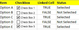
Checking a box changes the cell value to TRUE. Unchecking the box changes it to FALSE.
The checkbox moves with your data when you sort, filter, or insert rows. That’s because the checkbox is the cell.
Check the availability of native checkboxes in the table below.
| Platform | Native Checkboxes (Yes / No) |
| Microsoft 365 (Windows) | Yes |
| Microsoft 365 (Mac) | Yes |
| Excel for the Web | Yes (native checkboxes visible. Legacy controls not supported) |
| Excel 2024 (perpetual license) | No |
| Excel 2021, 2019, 2016 | No |
Legacy checkboxes are checkboxes that float above the cell. Also known as floating checkboxes, they have been in existence since 1993 with the launch of Excel 5.0 and are available in every version since. Users without a Microsoft 365 subscription must use these form control checkboxes. Here’s what you need to know about legacy checkboxes in Excel.
Form controls float above the cell grid.
They don’t store any values by default. So, you will have to manually link each checkbox to a cell.
The checkboxes don’t move with the rows. So the checkboxes can become misaligned after you sort or filter your data.
Despite these limitations, you will still need them for sharing files with people using older versions of the spreadsheet software. This is because native checkboxes will unideally appear as plain text on their screens.
Read Also: How to Create Dashboard in Excel? A step-by-step Guide
As I mentioned before, adding checkboxes in Excel is very simple. So, let me tell you how to do so according to the spreadsheet software version you have.
Here’s how to insert native checkboxes in Excel.
Select the cell where you want the checkbox.
Go to the Insert tab > Cell Controls group > click Checkbox.
The first thing you have to do is select a range of cells to add checkboxes to.
Click the Checkbox button. These boxes appear in all selected cells.
To make it work for non-adjacent selections, press Ctrl while clicking cells. Then insert them.
Insert one checkbox.
Grab the fill handle and drag.
You can also use your favorite pair of Ctrl + C and Ctrl + V shortcut keys.
| The Shortcut Itself | What It Does |
| Spacebar | Toggle checkbox state |
| Delete | Clear cell / remove checkbox formatting |
Take a look at the formula bar. Checked checkboxes show TRUE. Unchecked checkboxes show FALSE.
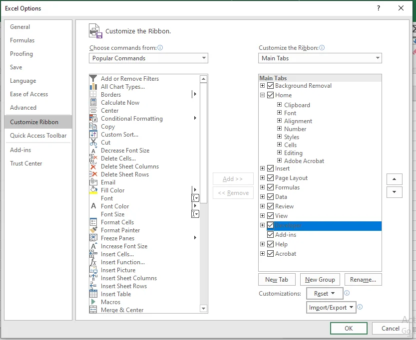
This is an extra step for users who have installed Excel 2016, 2019, 2021, or 2024 (perpetual). You must enable the Developer tab (hidden by default) before adding checkboxes in Excel. Fortunately, you will only have to do it once because the Developer tab stays in your ribbon after you enable it.
Navigate to File > Options > Customize Ribbon.
Check the Developer box in the right panel under “Main Tabs”.
Click OK.
Navigate to the Excel menu > Preferences > Ribbon & Toolbar.
Scroll all the way to the bottom of the Main Tabs list.
Check the Developer box.
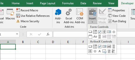
Click the Developer tab.
Click Insert in the Controls Group.
Click the Check Box icon under the Form Controls dropdown.
Click on the spreadsheet where you want the checkbox.
A checkbox is added with the default “Check Box 1” text. You can click and edit it or delete it if you only want the box.
Read Also: Excel ROUND(): A Quick Guide to Rounding in Excel
You will have to manually link checkboxes to cells in Excel using these simple steps. This is called explicit configuration of form controls. Simply put, Excel can read which checkbox belongs to which cell after you link them.
Right-click the checkbox.
Select Format Control.
Switch to the Control tab.
In the Cell Link field, enter a cell reference (like $B$2) or click the cell selector and click an empty cell.
Click OK.
| IGMGuru Tip |
|
During testing, copying a legacy checkbox without updating its linked cell caused multiple checkboxes to control the same TRUE/FALSE value. To avoid this issue, assign a unique linked cell to every form-control checkbox. Copying and pasting a form control checkbox will only waste your time because the copy will still refer to the first linked cell. You will end up manually updating each copy instead. |
Also Read: How to Remove Blank Rows in Excel?
You will have to make Excel formulas see legacy checkboxes indirectly. They will only see cell values, which won’t do anything. The linked cells make the formulas and checkboxes work together. Basically, the formulas will now understand properly that they have to function according to whether the checkbox has been ticked off or not.
| IGMGuru Tip |
| Putting linked cells next to a column near your checkboxes makes it easy for the formulas to read them. Ensure to hide them, so that the interface is not filled with messy TRUE / FALSE values. |
So far, I have talked about the importance of linked cells, Excel formulas, and how they work together. This section covers how it practically functions.
Keeping track of checked and unchecked checkboxes in Excel can be complicated in the rush of things. Especially if you have multiple boxes all over the worksheet. You can do this using the IF() formula.
=IF (A2=TRUE, “Complete”, “Pending”)
=IF (A2, “Complete”, “Pending”)
You can use the syntax you are comfortable with. Excel works with both.
Practical Examples:
| The Formula Itself | What it Does |
| =IF(A2=TRUE, “Done”, “”) | Show “Done” only when checked |
| =IF(A2, C2*0.1, 0) | Calculate 10% bonus when checked |
| = IF(A2=TRUE, C2*(1-0.2), C2) | Apply 20% discount when checked |
Checkboxes are the most useful when it comes to making important decisions. That’s because they simplify everything since users click boxes instead of typing conditions. Here are a few more real world examples:
A budget tracker will apply various tax rates based on your choices.
A project planner will only calculate resources for tasks whose checkboxes have been ticked off.
The IF() function will only tell you whether a checkbox is checked or not. However, what if you also want to know the number of checked and unchecked checkboxes in Excel? The COUNTIF () function is exactly what you require.Let me give you the Excel formula for counting checked boxes first.
=COUNTIF(A2:A20, TRUE)
| IGMGuru Tip |
| You can reference native checkbox columns directly. However, you must reference the linked cells for form controls. Also, don’t use the text values “TRUE” and “FALSE”. Excel will read them as plain text. |
Let me wrap up this section with the formula to count unchecked boxes.
=COUNTIF (A2:A20, FALSE)
Read Also: How to Find Standard Deviation in Excel?
Here are some real-life use cases of counting checkboxes in Excel.
Here’s the formula.
=COUNTIF(A2:A20, TRUE) / COUNTA(A2:A20)
All you have to do now is format the result cell as a percentage. Follow these simple steps to get the desired format.
Select the cell containing the result.
Navigate to the Home tab.
Look for the % (Percent Style) icon in the Number Group.
Click on it.
Press Ctrl + Shift + % if you are in a hurry.
The COUNTA() function counts non-empty cells. This way, the percentage value will still be right even if you have empty rows.
Consider this simple formula that calculates total items minus completed items.
=COUNTA(A2:A20) - COUNTIF(A2:A20, TRUE)
The resulting value will be the remaining items to complete.
Using this formula will perform addition of numbers in column B for the corresponding checked values in column A. Basically, what you are doing is instructing Excel formulas to coordinate with checkboxes. This restricts Excel to only sum numbers in columns where the checkbox is checked.
Also Explore: Pie Chart in Excel
This is quite helpful when you have bulk data. I am talking about 10s and 1000s of tasks. In such cases, looking for tick marks will waste your time. Conditional formatting helps users quickly understand pending and completed tasks.
Following these simple steps will highlight checked rows.
Select the range of cells you want to format (like A2:D20 for your entire data area).
Go to Home > Conditional Formatting > New Rule.
Choose “Use a formula to determine which cells to format”.
Enter the formula: =$A2=TRUE.
Click Format > choose a fill color.
Click OK twice.
Following these simple steps will strikethrough checked rows.
Choose the task description column (like B2:B20).
Navigate to Home > Conditional Formatting > New Rule.
Select “Use a formula to determine which cells to format”.
Enter the formula: =$A2=TRUE.
Click Format > Font tab.
Check Strikethrough.
Click OK twice.
| IGMGuru Tip |
| Combining multiple effects in a single rule is also possible. Just select all filters you need before clicking okay. |
Also Read: How to Compare Two Columns in Excel?
Removing or deleting the checkboxes in Excel is even simpler. You may want to only delete the formatting or remove everything according to your needs. I have covered everything in this section.
You can either delete the checkbox formatting only or delete everything. I have covered both methods here.
This will only make the checkbox icon go away. However, the TRUE / FALSE values will stay in their cells. This is the most reliable way to just get rid of the checkbox.
Select the cells containing checkboxes.
Navigate to Home > Clear > Clear Formats.
Following these steps will remove everything. Now Excel will consider whatever you type in the cells as plain text values.
Select the cells and press Delete to clear both the formatting and content.
Use Home > Clear > Clear All to remove everything.
Form control checkboxes in Excel float above the cells. Removing them becomes slightly different. However, it’s even simpler than deleting native checkboxes.
This method is slightly time-consuming because you will have to repeat these steps for every checkbox.
Ctrl + click the checkbox to select it.
Press Delete.
Here’s how to delete all checkboxes at once.
Navigate to Home > Find & Select > Selection Pane.
View and select specific objects by name. The object name is the name of the checkbox in our case. For example, “Check Box 1”.
Press Delete.
Their cell links and values still remain even after the legacy checkboxes are gone. This can cause big issues like:
The linked cells will keep their last values. This can be checked or unchecked.
Clicking on and around the cell where the checkbox was will do absolutely nothing.
Conditional formatting and formulas that relied on those cells will become static.
So, it is best practice to manually clear the cell links before further editing your Excel worksheet.
Read Also: Excel Formulas (Basic to Advanced)
You might run into some of these common problems when adding checkboxes in Excel. This section covers these issues and the simplest ways to fix them.
The most common issue is that you can’t find the checkbox option anywhere. This is most probably due to an older version of Excel on your system. You can check the software version under File > Account. If it’s not Microsoft 365, then you will have to use the developer method.
On the other hand, it is best practice to keep your Microsoft 365 subscription updated. Navigate to File > Account > Update Options > Update Now. You will always see the checkbox option as visible that way.
Someone might tell you that they only see TRUE / FALSE values in the worksheet you shared instead of checkboxes. This is because they are using an older version of Excel that doesn’t support native checkboxes. Another possibility is that they might not have updated their Microsoft 365 subscription.
The best practice is to create form control checkboxes (supported in every version of Excel) in spreadsheets you wish to share. Everyone can access the checkboxes without any confusion that way.
The solution for this issue changes according to the types of checkboxes in Excel.
Verify that the formula bar shows TRUE / FALSE values on cell selection.
If you have a TRUE / FALSE returning formula associated with a checkbox’s cell, it will only display the result. You can’t manually toggle it.
Right-click > Format Control > Verify the Cell Link field has a valid reference.
Each checkbox requires a unique cell link.
Cell links can’t refer to cells with formulas.
This is due to wrong instructions for the Excel version you are using. What I mean here is that each tutorial follows either the native or developer version. So, you must understand the differences first.
| Indicator | Native Checkbox | Form Control |
| Click behavior | Selects the cell | Toggles or selects the control |
| Formula bar | Shows TRUE / FALSE | Shows nothing (checkbox related) |
| Sizing handles | None visible | Appear when Ctrl + clicked |
| Right-click | Standard cell menu | Includes “assign macro” |
Follow the right method once you're clear on the confusion.
Also Explore: How to Use HLOOKUP Function?
The wise say that prevention is better than cure. Thus, it’s better to use these best practices for using checkboxes in Excel than to run into common problems time and again.
Use native checkboxes if you have a Microsoft 365 subscription and you don’t plan to share the worksheet with anyone.
In my testing, native checkboxes took less than a minute to add to a 50-row checklist and worked reliably with sorting, filtering, and formulas. For most Microsoft 365 users, they are significantly easier to manage than legacy form controls.
Otherwise, you have to use the developer method.
Linking cells is a must when using the developer method. I recommend that you place the links next to the column with checkboxes and hide them. This keeps the interface free of any cluster while your formulas can still access the data.
Think twice before copying a formula. Test it first to see if everything is working fine. Otherwise, you will waste time correcting the same error in multiple cells.
Form controls increase the file size and slow things down. Use native checkboxes if you still need to place many checkboxes because they are not separate objects. Another option for you is to place legacy checkboxes in Excel strategically.
Let them know the types of checkboxes used and the cell link location if you have shared your file with someone else. The best way to do so is to add simple comments.
Using checkboxes in your Excel spreadsheets makes the data interact with one another. The checkboxes can either be native to Microsoft 365 or they can be older controls that already existed prior. Regardless of which checkboxes are used, either type of checkbox helps people keep track of their activities, automate their calculations, and make data visibility higher.
Ans. You either have an older version of Excel or your Microsoft 365 version is outdated. I have already given the solutions in the article above. You can check them out.
Ans. Yes. You can change the checkbox’s formatting. This includes its font, fill color, borders, and alignment. However, there are limited customization options available in the checkbox symbol for the newer Microsoft 365 in-cell checkbox feature.
Ans. To create a checklist in Microsoft Excel, follow these simple steps.
Create the list that you want to convert to a checklist first.
Once you are done with that, add a checkbox to each row in your list.
Next, you need to enter the tasks next to each of them.
If you want, you can also use formulas to automatically change the statuses of the task statuses.