Are you struggling to remember which Excel formula to use and when? You’re not alone. I have seen many beginners with the same doubt. Once you clear this doubt, it will save you hours of manual work and prevent costly mistakes. It will be a shining star to your skill set. But the question is how.
Don’t worry! This guide covers the most important Excel formulas list, including basic Excel formulas, advanced Excel formulas, and practical examples for real-world use. Instead of just memorizing functions, you’ll understand how to actually use them in reports, dashboards, and everyday tasks. Whether you’re a beginner or improving your skills, this guide will help you work faster and smarter with Excel.
Excel formulas are expressions used in Microsoft Excel to perform calculations, analyze data, and automate tasks. They always start with an equal sign (=) and use functions, operators, and cell references to return results. One of the biggest advantages of using these formulas is that they update automatically. When the source data changes, Excel recalculates the result instantly, reducing manual effort and minimizing errors in spreadsheets.
For instance, if you type =A1 + B1, Excel will add the values in cells A1 and B1 and show the result in the cell where the formula is typed. In case you change the values in the A1 and B1 cells, the formula will automatically update the value.
This was just a basic example. Spreadsheet formulas go way beyond basic arithmetic. They can find matches, handle errors, manipulate text and dates, and even connect data from different sheets or workbooks. Once you get comfortable with a handful of functions, you'll be able to automate repetitive tasks and deliver cleaner, faster reports.
In real-world spreadsheet projects, formulas are rarely used in isolation. Analysts often combine logical, lookup, and error-handling formulas to clean data, validate inputs, and automate repetitive checks. Using the right formula structure can significantly reduce manual effort and spreadsheet errors.

Before exploring individual formulas, let’s explore how Excel formulas are grouped. The category helps you choose the right formula that matches and intent.
| Category | Formulas | Common Use Areas |
| Basic & Math | SUM, AVERAGE, COUNT, MIN, MAX, ROUND, ABS | Calculations |
| Logical | IF, AND, OR, NOT, IFS, SWITCH | Conditions, rules |
| Conditional | SUMIF, COUNTIF, AVERAGEIF, SUMIFS, COUNTIFS | Criteria-based analysis |
| Lookup & Reference | XLOOKUP, VLOOKUP, INDEX, MATCH, XMATCH, OFFSET | Data retrieval |
| Text | CONCAT, TEXTJOIN, LEFT, RIGHT, MID, LEN, TRIM, SUBSTITUTE | Text cleanup |
| Date & Time | TODAY, NOW, DATE, DATEDIF, YEAR, MONTH, EOMONTH | Time analysis |
| Error Handling | IFERROR, IFNA, ISERROR, ISNA, ISNUMBER | Error control |
| Statistical | MEDIAN, MODE, STDEV, RANK, PERCENTILE | Data analysis |
| Dynamic / Advanced | FILTER, SORT, UNIQUE, TAKE, DROP, LET | Modern Excel |
Using Excel formulas follows a simple and consistent process across all Excel versions. You can get confused as a beginner at first, but trust me 30 to 40 minutes is all it takes to be comfortable with these functions. You just have to learn their syntax and how to use them. The way of using a formula will not be the same every time due to different syntax, but the following steps are universal:
You need to explore each formula individually to understand its syntax perfectly and know how to use it.
Related Article: How to Use Power Query in Excel?
Key Takeaway: Basic and Math formulas form the foundation of Excel. Mastering functions like SUM, AVERAGE, and ROUND helps you perform accurate calculations and build reliable spreadsheets for everyday tasks.
| Formula | Category | Purpose |
| SUM | Basic & Math | Adds numbers |
| AVERAGE | Basic & Math | Finds mean |
| COUNT | Basic & Math | Counts numeric cells |
| MIN | Basic & Math | Smallest value |
| MAX | Basic & Math | Largest value |
| ROUND | Basic & Math | Rounds numbers |
| ABS | Basic & Math | Absolute value |
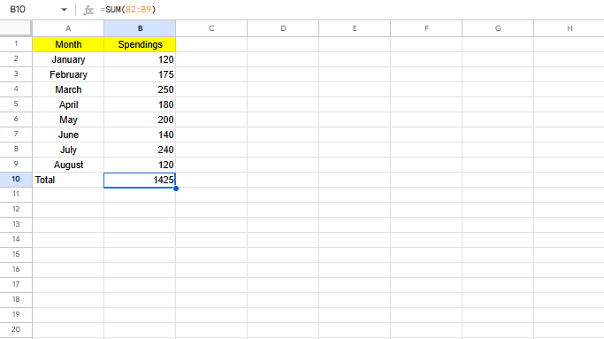
1. SUM adds a range of numeric values together. Use this formula when you need to calculate totals such as sales, expenses, or scores. It is commonly used to calculate totals such as sales, expenses, or scores.
|
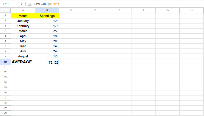
2. AVERAGE calculates the mean value of a range. Use this formula when you want to analyze overall performance or trends. This formula is useful for analyzing overall performance or trends.
|
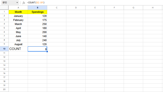
3. COUNT counts only the cells that contain numeric values. Use this formula when you need to count numeric entries in a dataset. It ignores text and blank cells, making it reliable for structured data.
Note: COUNT ignores text values. Use COUNTA if you want to count non-empty cells including text.
|
4. MIN returns the smallest number from a range. It is often used to find lowest scores or minimum costs.
|

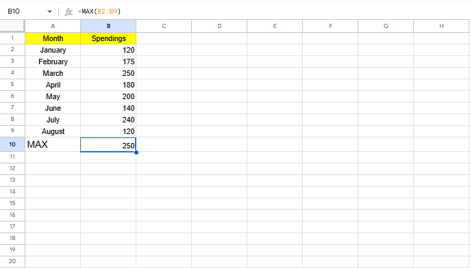
5. MAX returns the largest number from a range. This formula helps identify peak values, such as the highest sales or best performance.
|
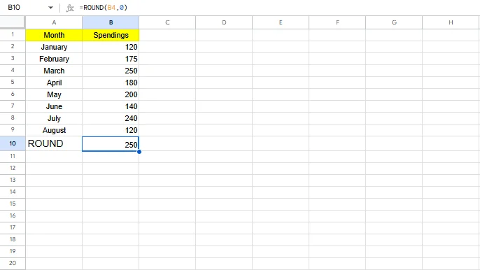
6. ROUND rounds a number to a specified number of digits. It is useful for financial reports where consistent formatting is required.
|
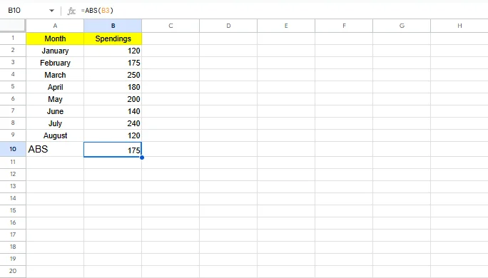
7. ABS converts negative numbers into positive values. It is commonly used in variance and difference calculations.
|
Logical formulas allow Excel to evaluate conditions and return results based on TRUE or FALSE outcomes. They are widely used in validations, grading systems, and automated decision-making.
| Category | Formulas | Common Use Areas |
| IF | Logical | Conditional output |
| AND | Logical | All conditions true |
| OR | Logical | Any condition true |
| NOT | Logical | Reverse logic |
| IFS | Logical | Multiple conditions |
| SWITCH | Logical | Value-based logic |
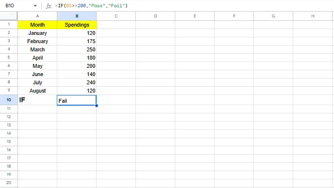
8. IF checks a condition and returns one value if the condition is true and another if it is false. Use this formula when you need to apply decision-based logic in your data. It is one of the most used Excel formulas.
|
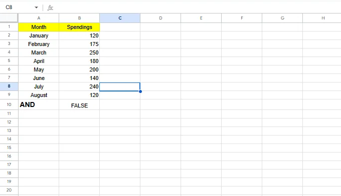
9. AND returns TRUE only if all specified conditions are true. It is often combined with IF for stricter rules.
|
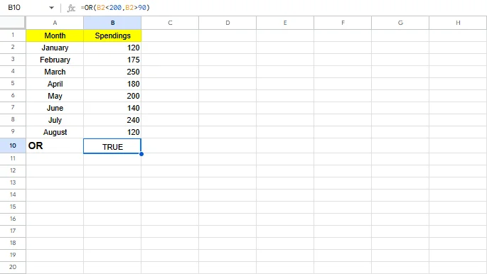
10. OR returns TRUE if at least one condition is true. This is useful when multiple criteria can qualify a result.
|
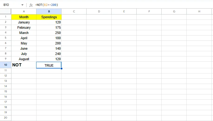
11. NOT reverses the result of a logical test. It is helpful when excluding specific conditions.
|
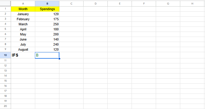
12. IFS evaluates multiple conditions in sequence without nested IF statements. It improves formula readability and maintenance.
|
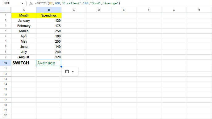
13. SWITCH compares a value against multiple cases and returns a matching result. It is ideal for fixed-value mappings.
|
Conditional formulas apply calculations only when specific criteria are met. These formulas are essential for filtered reporting and segmented analysis.
| Category | Formulas | Common Use Areas |
| SUMIF | Conditional | Conditional sum |
| COUNTIF | Conditional | Conditional count |
| AVERAGEIF | Conditional | Conditional average |
| SUMIFS | Conditional | Multi-condition sum |
| COUNTIFS | Conditional | Multi-condition count |
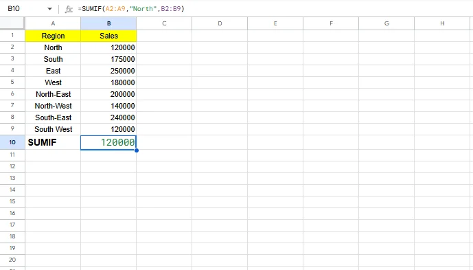
14. SUMIF adds values that meet a single condition. It is useful for calculating totals by category.
|
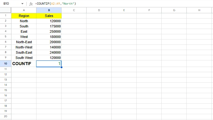
15. COUNTIF counts how many cells meet a specific condition. It is commonly used for tracking status or attendance.
|
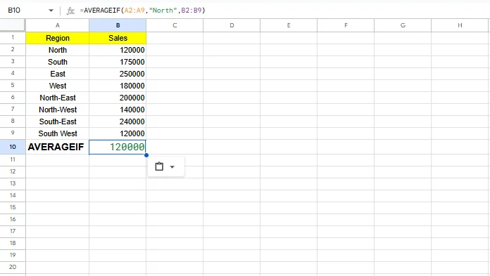
16. AVERAGEIF calculates the average of values that meet a condition. This helps analyze group-based performance.
|
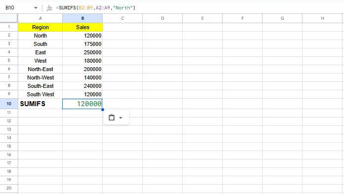
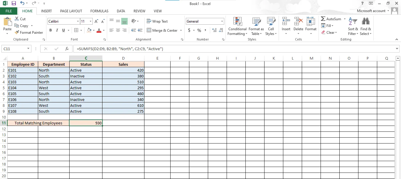
17. SUMIFS adds values based on one or more conditions across different ranges. It is ideal for complex business reports.
|
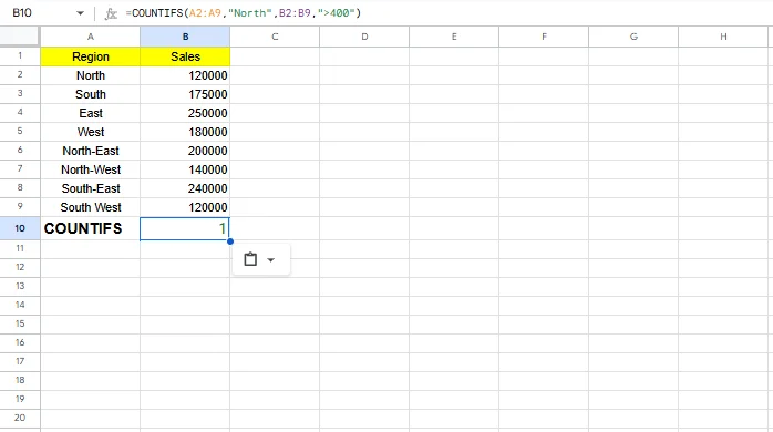
18. COUNTIFS counts cells that meet multiple criteria. It is useful for multi-filter analysis.
|
Key Takeaway: Lookup formulas like XLOOKUP and INDEX/MATCH allow you to retrieve data dynamically from large tables. In modern Excel versions, XLOOKUP is preferred for its flexibility and cleaner syntax.
| Category | Formulas | Common Use Areas |
| XLOOKUP | Lookup | Modern lookup |
| VLOOKUP | Lookup | Vertical lookup |
| INDEX | Lookup | Value by position |
| MATCH | Lookup | Position lookup |
| XMATCH | Lookup | Advanced match |
| OFFSET | Lookup | Dynamic range |
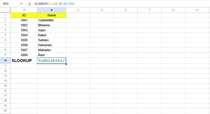
19. XLOOKUP searches for a value and returns a matching result from another range. It is flexible and replaces older lookup functions.
|
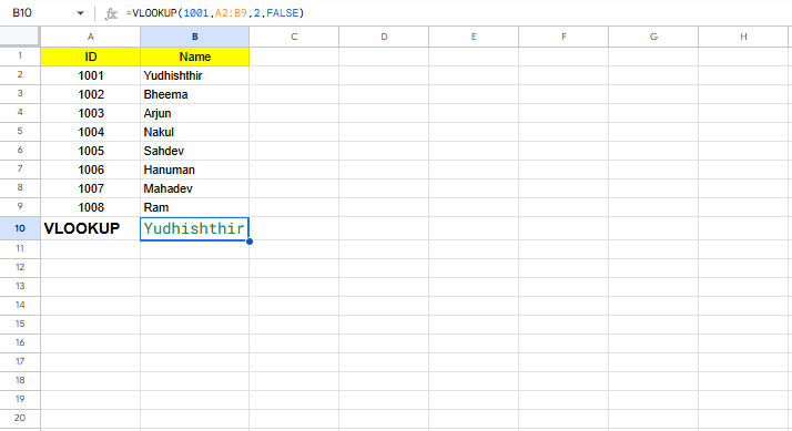
20. VLOOKUP searches vertically in the first column of a table. Use this formula when you need to find and retrieve data from structured tables. It is widely used but has column limitations.
|
21. INDEX returns a value from a specified position in a range. It is often combined with MATCH.
|

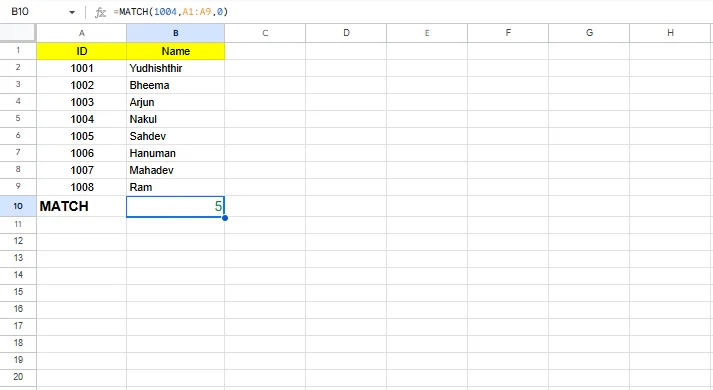
22. MATCH finds the position of a value in a range. It enables dynamic lookup systems.
|
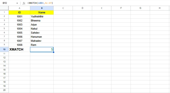
23. XMATCH is an advanced version of MATCH with more flexibility. It works well with modern Excel features.
|
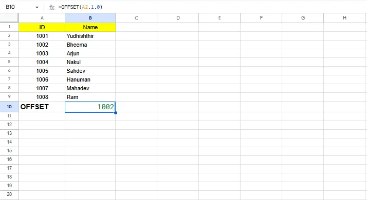
24. OFFSET returns a reference offset from a starting point. It is useful for dynamic ranges.
Performance Tip: OFFSET is a volatile function, meaning it recalculates whenever Excel recalculates. In large or complex spreadsheets, using INDEX with dynamic arrays often provides better performance and stability.
|
Text formulas help clean, extract, and combine text data, which is common in real-world spreadsheets.
| Category | Formulas | Common Use Areas |
| CONCAT | Text | Join text |
| TEXTJOIN | Text | Join with a delimiter |
| LEFT | Text | Left characters |
| RIGHT | Text | Right characters |
| MID | Text | Middle characters |
| LEN | Text | Text length |
| TRIM | Text | Remove spaces |
| SUBSTITUTE | Text | Replace text |
25. CONCAT joins text from multiple cells or strings into one. It replaces the older CONCATENATE function.
|
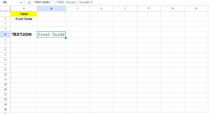
26. TEXTJOIN combines text using a delimiter and can ignore empty cells.
|
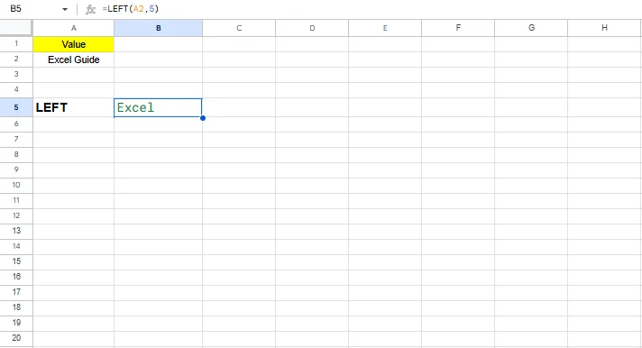
27. LEFT extracts a specified number of characters from the left side of the text.
|
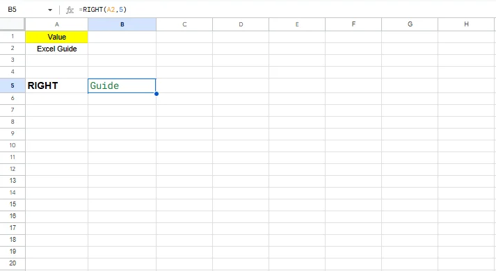
28. RIGHT extracts characters from the right side of the text.
|
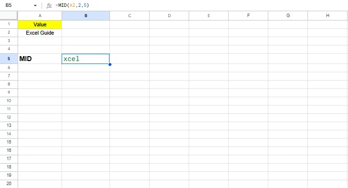
29. MID extracts text from the middle of a string.
|
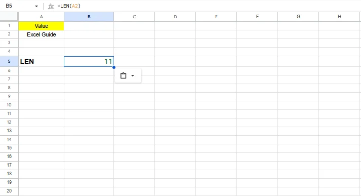
30. LEN returns the total number of characters in text.
|
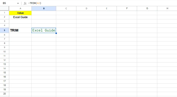
31. TRIM removes extra spaces except single spaces between words.
|
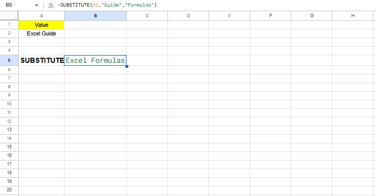
32. SUBSTITUTE replaces specific text with new text.
|
Date and Time formulas help manage schedules, calculate durations, and analyze time-based data. These formulas are widely used in project tracking, payroll, reporting periods, and deadline management.
| Category | Formulas | Common Use Areas |
| TODAY | Date & Time | Current date |
| NOW | Date & Time | Current date and time |
| DATE | Date & Time | Create a date |
| DATEDIF | Date & Time | Date difference |
| YEAR | Date & Time | Extract year |
| MONTH | Date & Time | Extract month |
| EOMONTH | Date & Time | End of month |
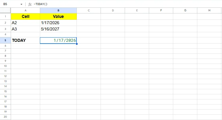
33. TODAY returns the current system date and updates automatically every day. It is useful for tracking deadlines, reports, and dynamic dashboards.
|
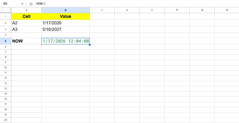
34. NOW returns the current date along with the current time. This formula is commonly used in time-sensitive tracking and logging.
|
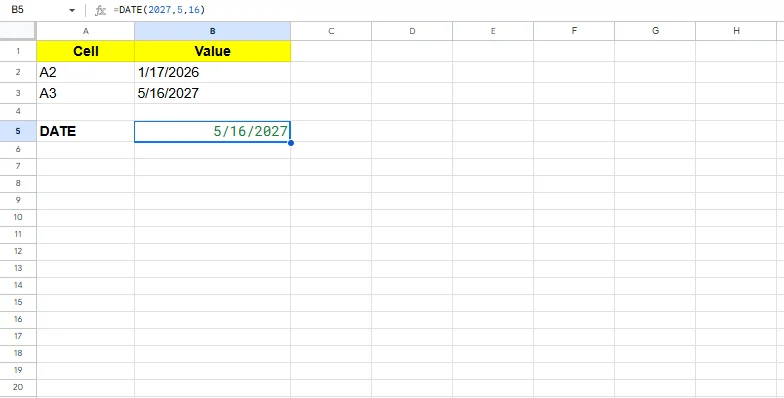
35. DATE creates a valid date using year, month, and day values. It helps avoid date formatting issues when combining date components.
|
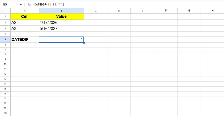
36. DATEDIF calculates the difference between two dates in days, months, or years using units such as "Y", "M", or "D". Although undocumented, DATEDIF is fully supported and widely used in Excel. It is useful for calculating age, tenure, or project duration.
|
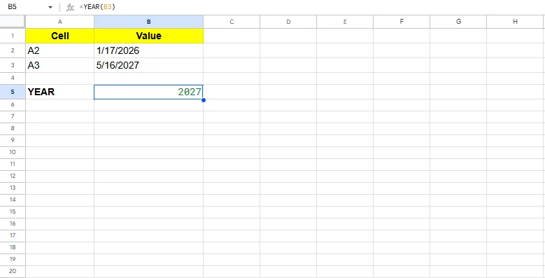
37. YEAR extracts the year from a given date. This is helpful when grouping or filtering data by year.
|
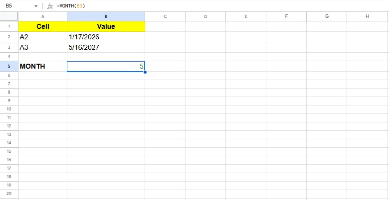
38. MONTH returns the month number from a date. It is commonly used in monthly trend analysis.
|
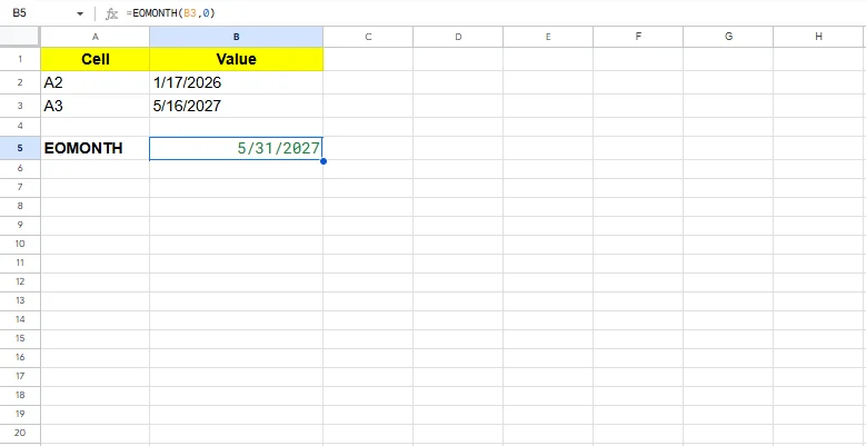
39. EOMONTH returns the last day of a specified month. This formula is useful for financial reporting and billing cycles.
|
Error-handling formulas keep spreadsheets clean and user-friendly by managing or detecting errors. These formulas prevent confusing error messages from appearing in reports.
| Category | Formulas | Common Use Areas |
| IFERROR | Error Handling | Replace errors |
| IFNA | Error Handling | Handle #N/A errors |
| ISERROR | Error Handling | Detect errors |
| ISNA | Error Handling | Detect N/A |
| ISNUMBER | Error Handling | Check numeric values |
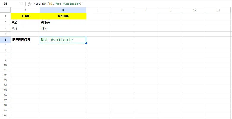
40. IFERROR replaces any formula error with a custom value. It is widely used to display clean outputs in dashboards.
|
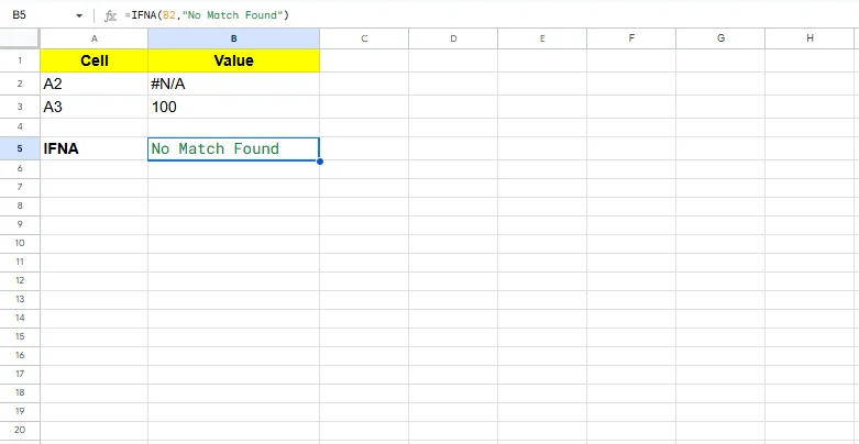
41. IFNA specifically handles #N/A errors without affecting other error types. It is useful in lookup formulas.
|
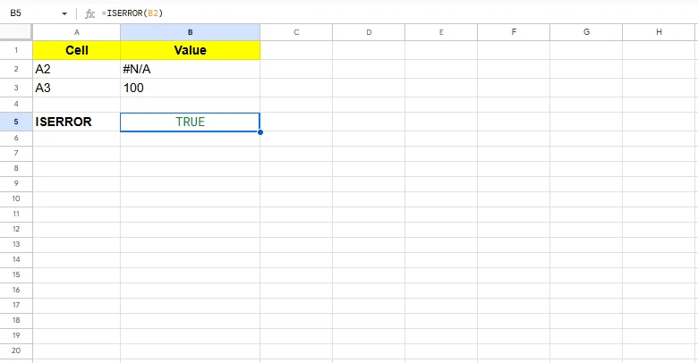
42. ISERROR checks whether a cell contains any error. It returns TRUE or FALSE.
|
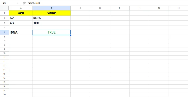
43. ISNA checks only for the #N/A error. This helps identify missing lookup results.
|
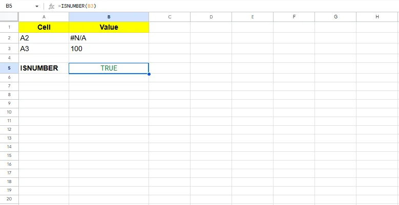
44. ISNUMBER checks whether a value is numeric. It is commonly used in data validation and cleaning.
|
Statistical formulas help analyze data distribution, rankings, and trends. These formulas are widely used in reporting, analytics, and decision-making.
| Category | Formulas | Common Use Areas |
| MEDIAN | Statistical | Middle value |
| MODE | Statistical | Most frequent value |
| STDEV | Statistical | Data spread |
| RANK | Statistical | Rank values |
| PERCENTILE | Statistical | Percent position |
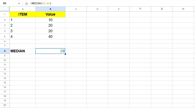
45. MEDIAN returns the middle value of a dataset. It is useful when outliers affect average values.
|
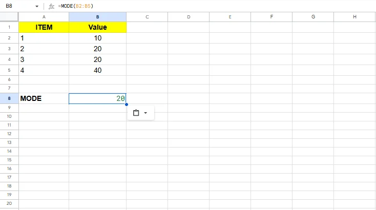
46. MODE returns the most frequently occurring value. It is useful for identifying common trends.
|
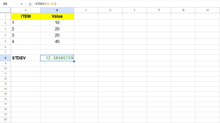
47. STDEV measures how much values deviate from the average. It is commonly used in risk and variability analysis.
Tip: In newer Excel versions, STDEV.S (sample) and STDEV.P (population) are preferred for more precise statistical analysis.
|
48. RANK assigns a rank to a value within a dataset. It is often used in performance comparisons.
|
![]()
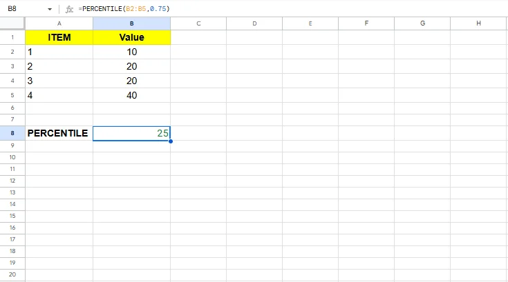
49. PERCENTILE returns the value at a given percentile. It is useful in distribution analysis.
|
Advanced and dynamic formulas enable modern Excel features such as dynamic arrays and optimized calculations. These formulas are essential for scalable and automated reports.
Note on Excel Versions: Dynamic array formulas such as FILTER, SORT, UNIQUE, and LET are available in Microsoft Excel 365 and newer versions. If you are using older Excel versions, some formulas may not be supported.
| Category | Formulas | Common Use Areas |
| FILTER | Advanced | Filter data dynamically |
| SORT | Advanced | Auto-sort data |
| UNIQUE | Advanced | Remove duplicates |
| LET | Advanced | Optimize formulas |
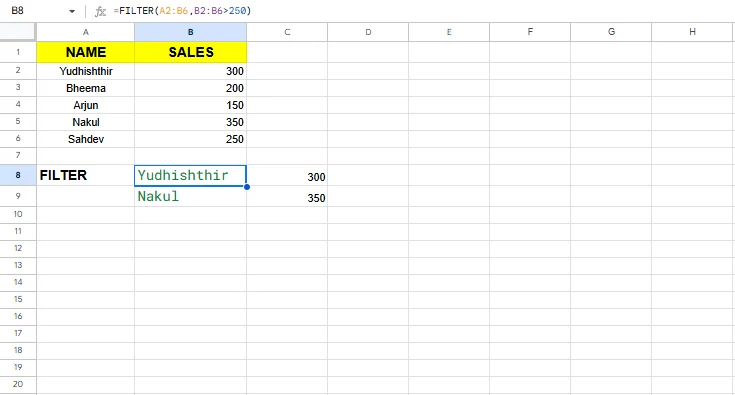
50. FILTER extracts rows that meet a condition and updates dynamically. It removes the need for helper columns.
|
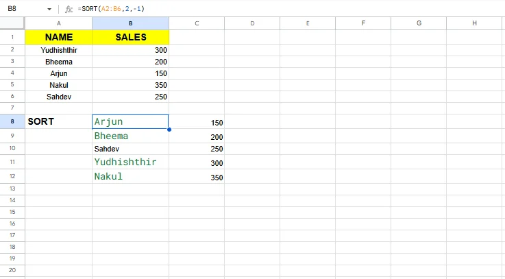
51. SORT automatically sorts data based on specified columns. It updates instantly when source data changes.
|
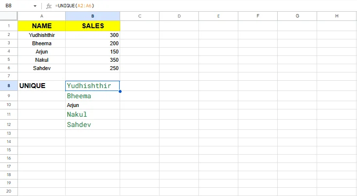
52. UNIQUE returns distinct values from a list. It is ideal for summary reports.
|
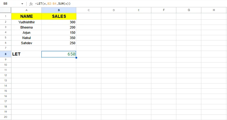
53. LET assigns names to calculations within a formula. It improves performance and readability.
|
Advanced Excel is not just about memorizing built-in functions. The real power starts when you begin creating your own formulas by combining operators, logical expressions and dynamic techniques. Custom formulas allow you to design calculations that match your exact business requirements instead of depending only on predefined functions.
These types of formulas are extremely useful in real-world projects, as the built-in ones are rarely used in isolation. Analysts also combine arithmetic operators, conditions and dynamic arrays to automate reports, reduce manual work and improve spreadsheet scalability. Let’s understand how you can create your own advanced Excel formulas step by step.
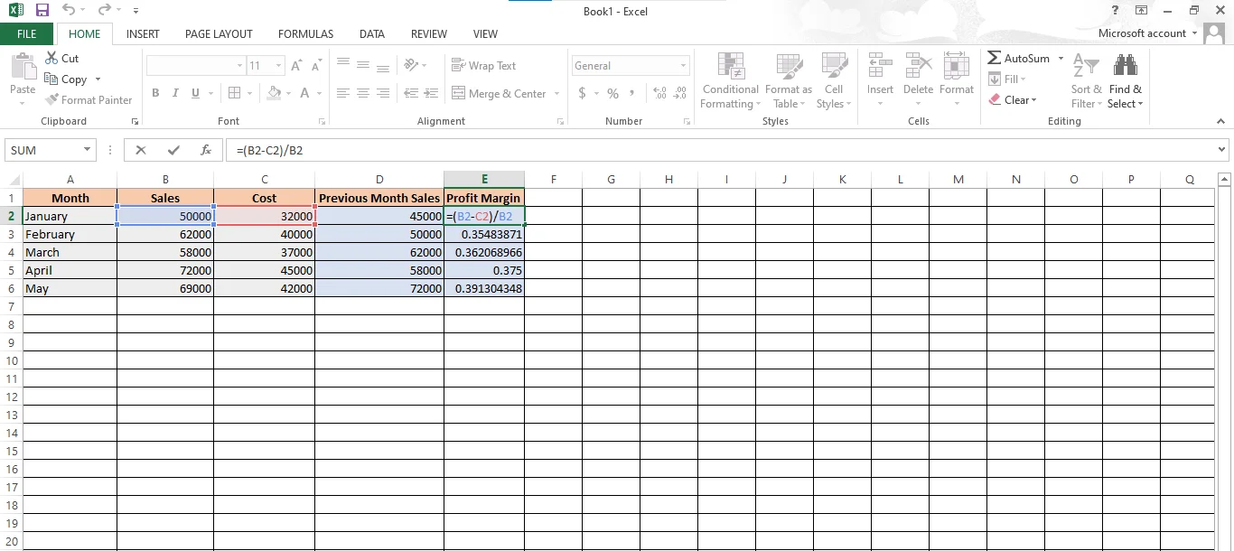
Excel formulas are not limited to functions like SUM or IF. You can create powerful custom calculations using arithmetic and logical operators. These formulas automatically update whenever the source data changes, which makes them ideal for dashboards and performance tracking. Common operator-based formulas:
|
|
|
|
|
These simple operator formulas form the foundation of advanced calculations. They are widely used in financial reporting, sales performance tracking, growth rate analysis and commission calculations. Let’s see an example of calculating profit margin using customized formulas:
Array formulas allow you to perform calculations on multiple values at once. This means you don’t have to process one cell at a time. These formulas will evaluate entire ranges and return either a single result or multiple results dynamically.
|
|
|
In Excel 365 and newer versions, array formulas “spill” results automatically into adjacent cells. In older Excel versions, some array formulas require pressing Ctrl + Shift + Enter to work properly. These functions are extremely useful for multi-condition analysis, dashboard automation and handling large datasets efficiently. Let’s understand them with an example of Employee Performance Tracking:
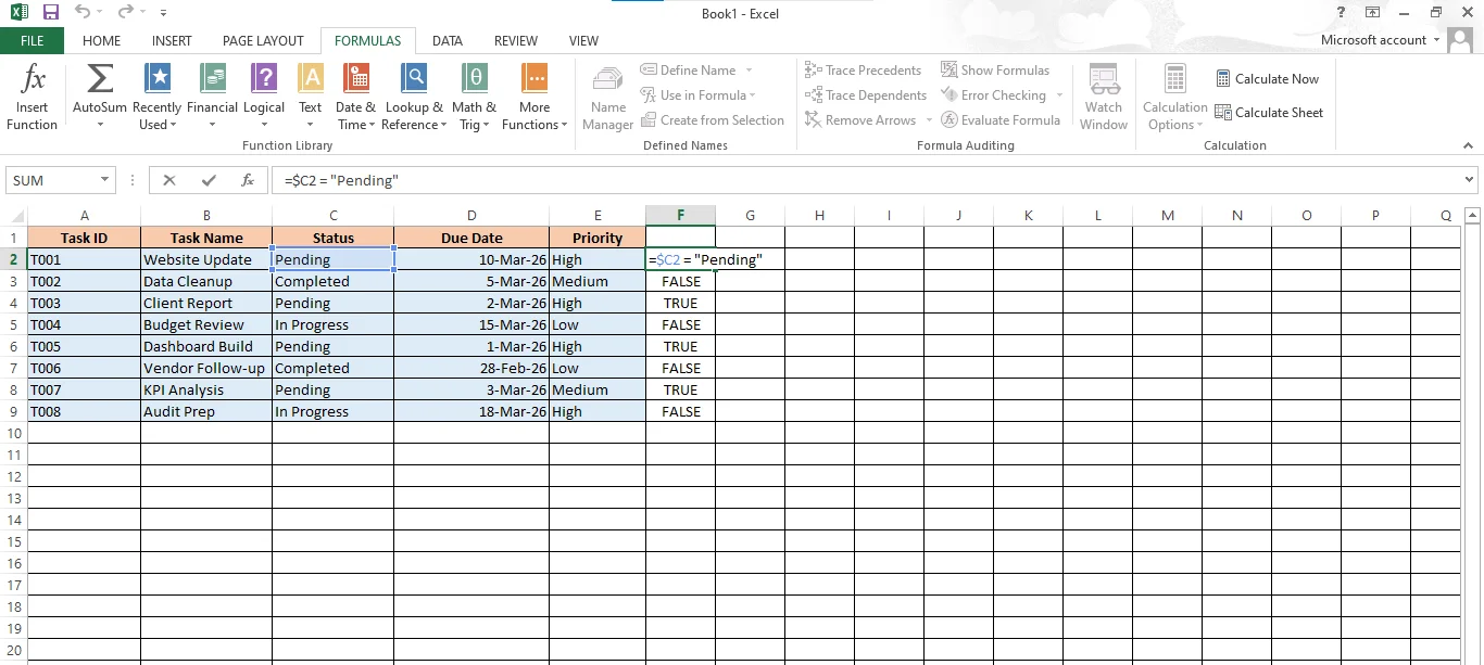
Advanced formula usage is not limited to calculation cells. You can also use formulas inside Conditional Formatting to create dynamic visual alerts. This helps you highlight important data automatically based on specific logic. How it works:
|
This formula highlights entire rows where column C contains the word “Pending”.
Formula-based conditional formatting adds intelligence to your spreadsheets. Instead of manually checking values, Excel visually signals important insights in real time. Let’s see an example:
The traditional formulas we have learned through this guide are not always helpful when used alone. It requires using different combinations of formulas to perform complicated calculations. The best part is that it is possible and easy. Let’s understand how with examples:
Example:
|
Here, the result will only be “Pass” if both conditions are true.
Example:
|
This helps you perform lookups only when a condition is met.
Example:
|
This ensures your spreadsheet looks clean and professional.
Microsoft Excel has evolved significantly in recent years, especially in Microsoft 365. Modern Excel now includes dynamic array formulas, text-processing functions, array transformation formulas, and even AI-powered capabilities. These formulas help users automate complex tasks, clean data faster, and build scalable reports without relying heavily on VBA or helper columns.
Many of these newer formulas are designed for modern data analysis workflows and are especially useful for dashboard creation, data cleaning, reporting automation, and business intelligence tasks. Let’s explore some of the most important modern Excel formulas introduced in recent Excel updates.
| Formula | Purpose | Common Use Areas |
| TEXTSPLIT | Split text dynamically | Data cleaning |
| TEXTBEFORE | Extract text before a delimiter | String extraction |
| TEXTAFTER | Extract text after a delimiter | Text processing |
| TAKE | Extract rows or columns | Dynamic reports |
| DROP | Remove rows or columns | Dataset cleanup |
| CHOOSECOLS | Select specific columns | Reporting |
| CHOOSEROWS | Select specific rows | Filtered analysis |
| TOCOL | Convert arrays into columns | Array transformation |
| TOROW | Convert arrays into rows | Data reshaping |
| HSTACK | Combine arrays horizontally | Dashboard building |
| VSTACK | Combine arrays vertically | Data consolidation |
| WRAPROWS | Wrap values into rows | Dynamic layouts |
| WRAPCOLS | Wrap values into columns | Structured formatting |
| REGEXEXTRACT | Extract text using patterns | Advanced text cleaning |
| REGEXREPLACE | Replace text using patterns | Data standardization |
| REGEXTEST | Validate text patterns | Input validation |
| GROUPBY | Group and aggregate data | Summary reporting |
| PIVOTBY | Create pivot-style summaries | Dynamic analytics |
| PY | Run Python in Excel | Advanced analytics |
| IMPORTCSV | Import CSV files dynamically | Automated reporting |
| IMPORTTEXT | Import text files dynamically | External data loading |
TEXTSPLIT separates text into multiple columns or rows using a delimiter. This is extremely useful when cleaning imported datasets.
|
TEXTBEFORE extracts text before a specific character or delimiter. It simplifies string parsing tasks.
|
TEXTAFTER extracts text appearing after a delimiter. It is commonly used for domain extraction and data cleanup.
|
TAKE returns a specified number of rows or columns from a dataset. This formula is useful for dynamic dashboards and preview tables.
|
DROP removes a specified number of rows or columns from a dataset dynamically.
|
REGEXEXTRACT extracts values using pattern matching. It is extremely powerful for advanced text processing.
|
GROUPBY creates grouped summaries directly with formulas instead of traditional Pivot Tables.
|
PY allows users to run Python code directly inside Excel. This feature is useful for machine learning, statistical analysis, and advanced data science workflows.
|
IMPORTCSV dynamically imports CSV files into Excel and updates them automatically when the source file changes.
|
IMPORTTEXT imports plain text files dynamically into Excel for automated processing workflows.
|
Important Note: Most of these modern formulas are available only in Microsoft Excel 365 and newer Excel versions. Some features may require the latest Microsoft 365 updates.
Modern Excel is moving toward AI-assisted and dynamic spreadsheet automation. Along with these formulas, Microsoft Copilot can now suggest formulas, explain calculations, generate reports, and automate spreadsheet tasks using natural language prompts. However, understanding the formulas manually is still essential for building reliable and scalable spreadsheets.
You have to be very careful while using these functions. A small mistake can lead to incorrect results or broken calculations. Here are some of the common errors to avoid that will save you time and frustration.
| Mistake | What Happens | Example | Solution |
| Incorrect Cell References | Wrong cell or range leads to incorrect results | Using A1:A5 instead of A1:A10 | Double-check references before applying formulas |
| Missing Parentheses | Changes the calculation order and gives the wrong output | =A1+B1*C1 instead of =(A1+B1)*C1 | Always use brackets to control calculations |
| Dividing by Zero (#DIV/0!) | An error occurs when dividing by an empty or zero value | =A1/B1 (when B1 is 0 or empty) | Use =IFERROR(A1/B1,"Error") |
| Wrong Data Type | Text values break numeric calculations | "100" treated as text instead of a number | Convert text to numbers using VALUE or formatting |
| Absolute vs Relative Reference | The formula changes incorrectly when dragged | A1 instead of $A$1 | Use $ to lock cells when needed |
| Lookup Errors (#N/A) | Value not found in lookup range | VLOOKUP returns #N/A | Ensure data matches or use IFNA/IFERROR |
| Extra Spaces in Data | Spaces cause lookup and text errors | "Excel " vs "Excel" | Use TRIM to remove extra spaces |
Excel formulas are the foundation of efficient spreadsheet work for data calculations, report creation, and effective communication with stakeholders. You can start with the core formulas and gradually move on to more advanced functions like INDEX/MATCH, TEXTJOIN and XLOOKUP to your toolbox. This guide covers essential Excel formulas used in real-world reporting, data analysis, automation, and interview preparation. By mastering these formulas, you can work faster, reduce errors, and build scalable spreadsheets with confidence.
In 2026, Excel formulas are increasingly supported by AI-powered features such as Copilot, which can suggest formulas, explain errors, and generate expressions based on natural language prompts. While AI improves productivity, understanding core Excel formulas remains essential for accuracy and control.
Explore Our Trending Articles
The most important Excel formulas include SUM, IF, VLOOKUP, XLOOKUP, COUNT, and CONCAT. These formulas are widely used in data analysis and reporting.
Beginners should start with basic Excel formulas like SUM, AVERAGE, COUNT, and IF before moving to advanced formulas like VLOOKUP and XLOOKUP.
Excel offers hundreds of built-in functions - typically 400+ to 500+, depending on your Excel version (Microsoft continually adds functions like XLOOKUP, TEXTSPLIT, etc.). For daily work, you only need a small subset of commonly used formulas.
To remove duplicates: select your range, go to the Data tab → click Remove Duplicates, choose the columns to check and confirm. Tip: always keep a backup or work on a copy before removing duplicates.
A simple Excel formula starts with a number = followed by arithmetic or functions. Example: =A1 + B1 or =SUM(A1:A5). Use parentheses to control the order of operations, like = (A1+B1) * C1.
If you have access to newer Excel versions (Office 365 / Excel 2019+), you prefer XLOOKUP() flexible, bi-directional lookups and easier syntax. Use INDEX/MATCH when working with legacy Excel or complex lookups.
Lock cells containing formulas (Format Cells → Protection → check Locked), then protect the sheet (Review → Protect Sheet). You can still allow certain actions, but locked cells cannot be edited without the password.
Most formulas work cross-platform. Avoid using Windows-only shortcuts in instructions; prefer menu paths (e.g., Insert → Table). Check date and regional formats (mm/dd/yyyy vs dd/mm/yyyy) when sharing sheets across regions.