Comparing two columns in Excel may sound like a simple task, but it quickly becomes challenging when you’re dealing with large datasets, repeated values or small mismatches that are easy to overlook. Whether you are checking customer lists, validating reports, or auditing business data, knowing how to compare two columns in Excel is an essential skill.
In this Excel tutorial, you’ll learn how to compare two columns in Excel using practical, real-world methods. We’ll explore everything from basic formulas for finding matches and mismatches to more advanced lookup techniques for identifying duplicates and inconsistencies. By the end of this guide, you’ll be able to confidently validate, clean, and audit your data, saving time and avoiding costly errors in your analysis and reports.

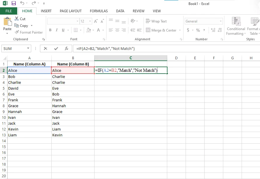
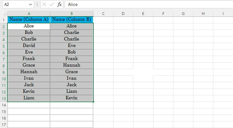
If you are looking for the fastest way to compare two columns in Excel, this simple formula-based method is the easiest place to start. It works well for small to medium datasets where values are aligned row by row, and you just want a quick yes-or-no comparison. While this approach is not ideal for complex data validation, it helps you instantly spot matches and mismatches without any advanced Excel knowledge.
Here’s how to compare two columns in Excel using quick steps:
1. Click on cell C2, insert the following formula, and hit the enter button.
|
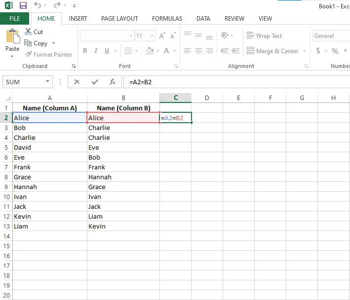
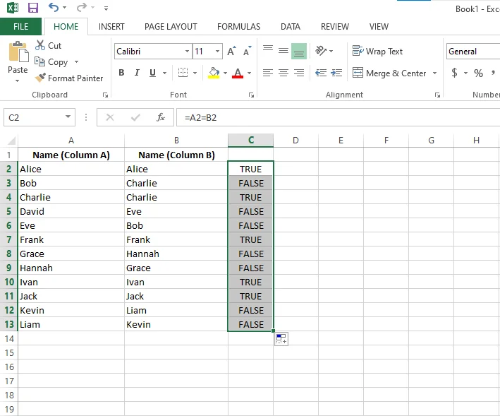
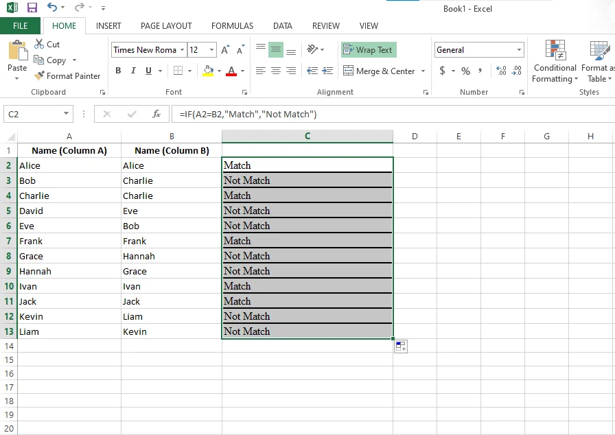
2. Drag the formula down to other rows. Excel will return TRUE if the values in both columns match and FALSE if they don’t. This quick solution is perfect when you need immediate results, but for larger datasets or deeper analysis, more efficient and advanced methods are discussed in the next sections.
Excel offers several comparison methods, each with different advantages depending on the complexity of the data you have at hand. You need to know every method to become a proficient data professional. Let's explore all of these methods one by one:
1. Click on cell C2, insert the following formula and hit the enter button.
|
2. Drag the formula down to other rows. The following results you will get:
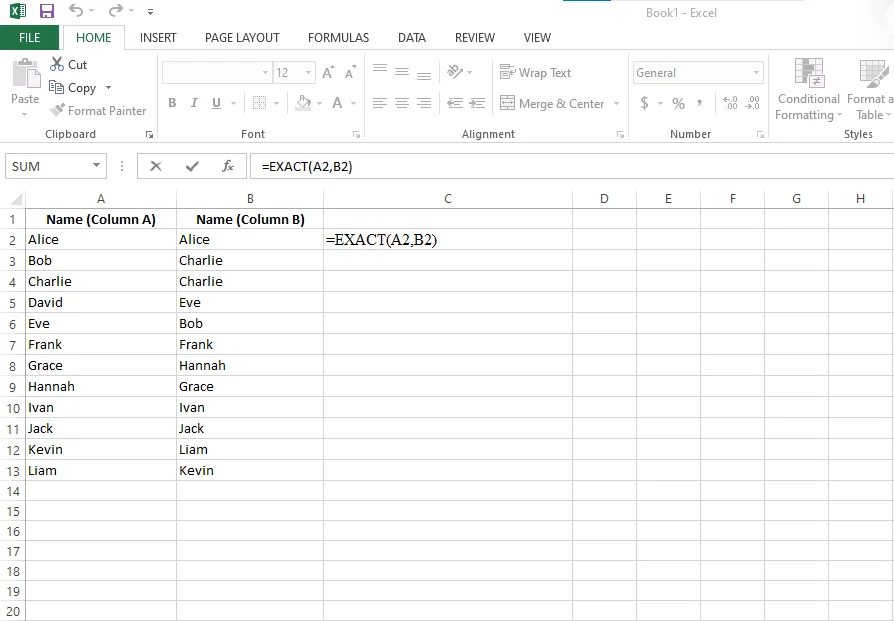
1. Click on cell C2, insert the following formula and hit the enter button.
|
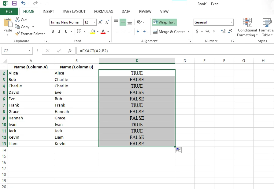
2. Drag the formula cell down to make the same changes in other cells. What will happen:
Unlike the equals (=) operator, the EXACT() function is case-sensitive. The equals operator ignores uppercase and lowercase differences, but EXACT() treats "Excel" and "excel" as different values.
1. Click on C2 and type the following formula:
|
2. Drag the formula cell to the last row of data and your sheet will look like this:
Note: Using entire column references like A:A or B:B is generally safe in modern versions of Excel. However, in very large datasets (100,000+ rows) or when using complex formulas, limiting the range to specific rows (for example B2:B5000) can improve performance.
If you are using Excel 365 or Excel 2021 and later versions, XLOOKUP is a more powerful and flexible alternative to VLOOKUP. It is easier to use and does not require column index numbers.
1. Click on cell C2 and type the following formula:
|
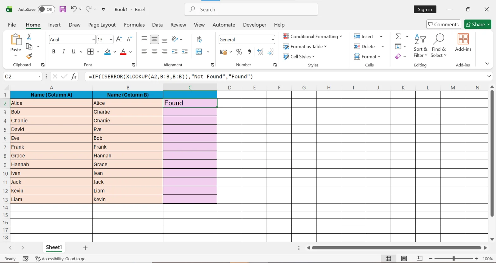
2. Press Enter and drag the formula down.
Excel will return:
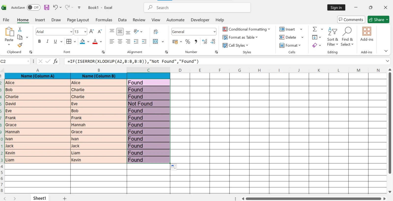
XLOOKUP is recommended for modern Excel users because it is more efficient and flexible than VLOOKUP.
1. Select column A from A2 to wherever your data ends.
2. Go to Home → Conditional Formatting → New Rule → Use a formula to determine which cells to format. Enter the following formula:
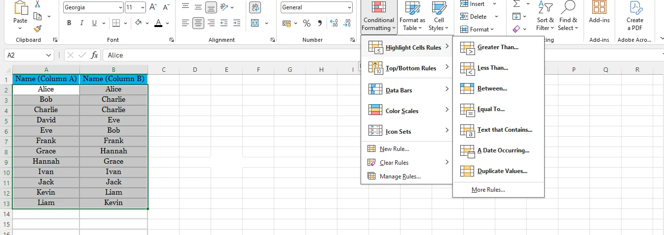
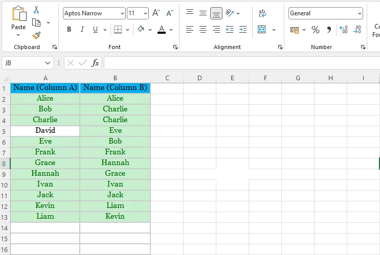
3. Click Format, choose a highlight color, and press OK. Now Excel will highlight values in column A that also exist in column B.
Read Also: How to Remove Blank Rows in Excel?
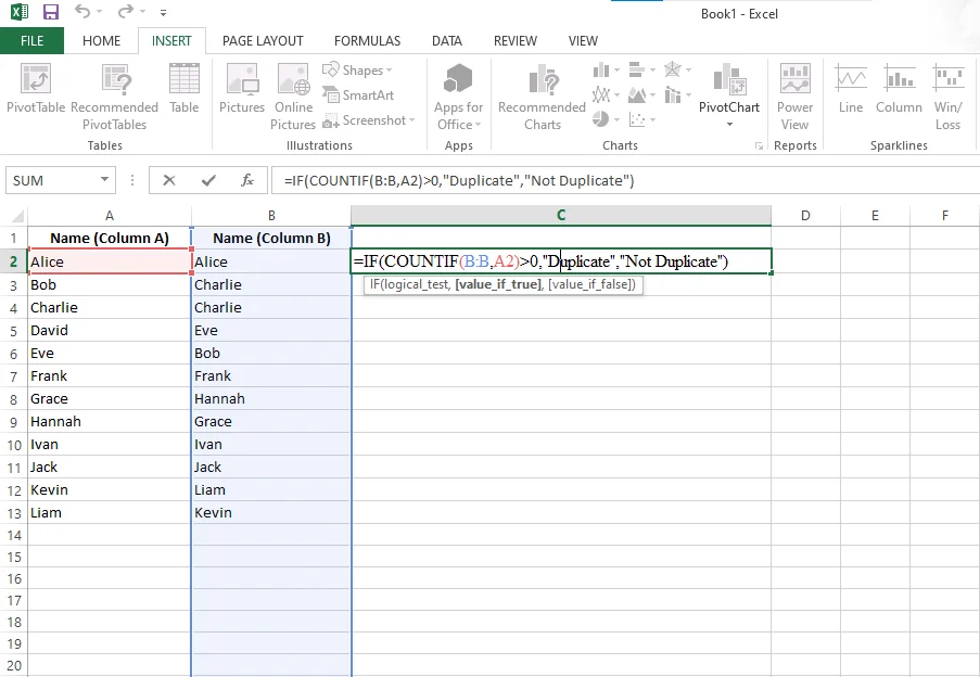
Finding duplicates is another reason why we will have to compare two columns in Excel. Well, it is a part of data cleansing methods that include using different formulas. let's understand how:
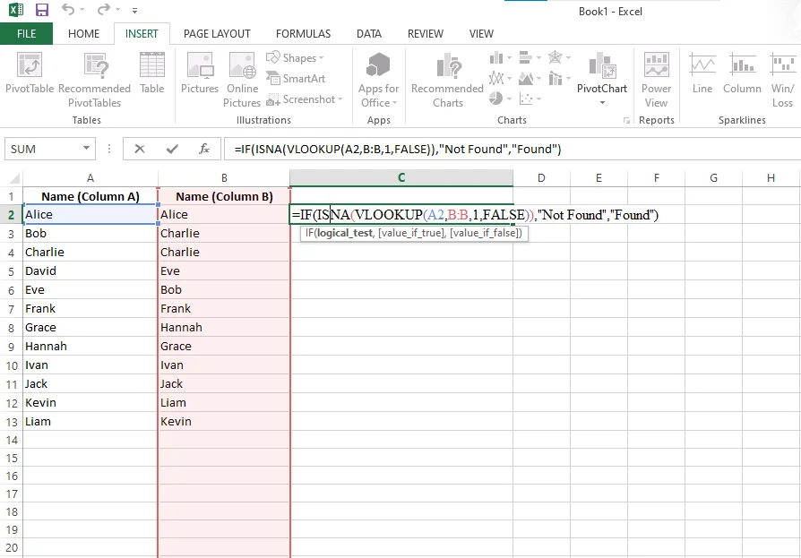
1. Click on C2 and type the following formula and press the Enter button.
|
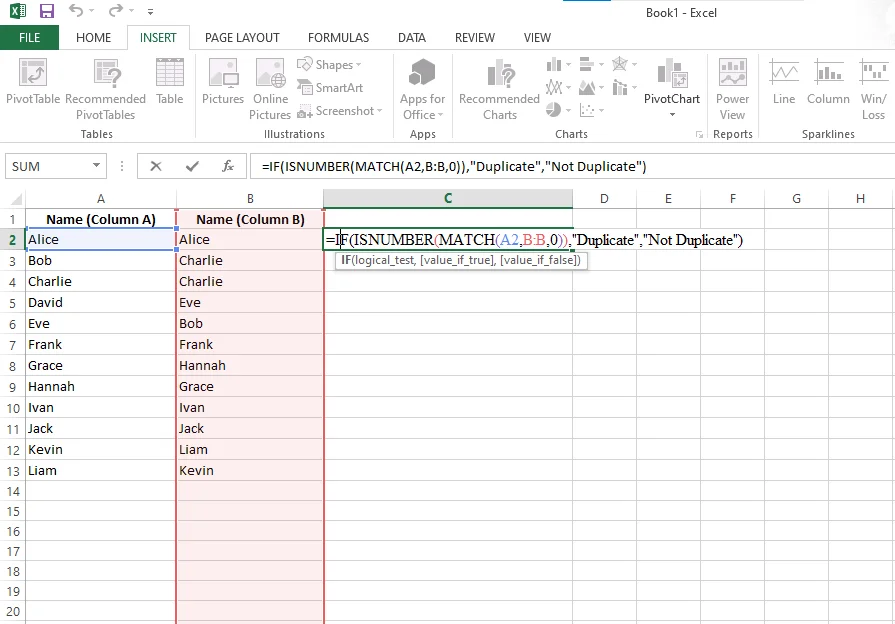
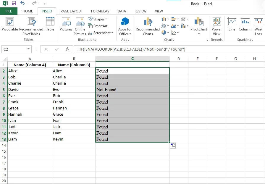
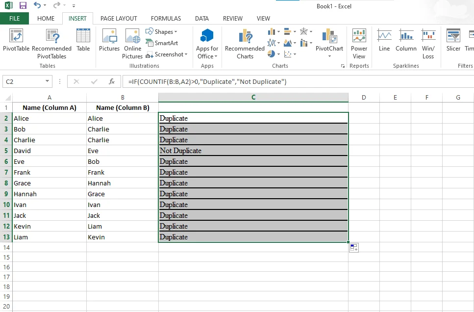
2. Now Click on C2, drag the small blue square (fill handle) down to the last row. Now each row is checked automatically using the applied formula just like the reference image:

1. Click on C2 and type this formula and press the enter button:
|
2. Click on C2 and drag the small blue square down. Your data will look like this:
In Excel 365, you can use dynamic array formulas to directly extract values that are missing in another column.
To show values in Column A that do not exist in Column B:
|
This formula automatically returns a list of values that are present in Column A but missing in Column B.
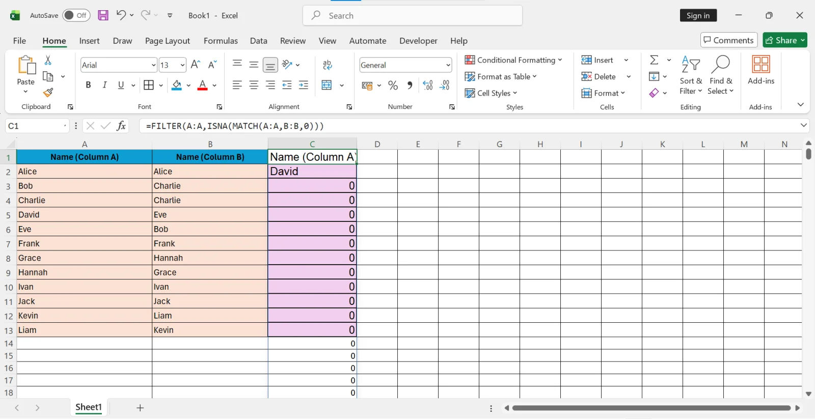
The FILTER function is useful when you want a separate clean list of unmatched values instead of just labeling rows.
For very large datasets, Power Query is the most professional and reliable way to compare columns.
1. Select your data and convert it into a Table (Ctrl + T).
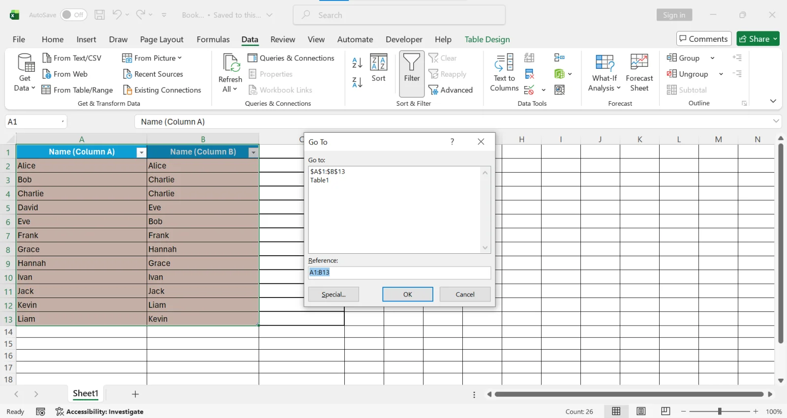
2. Go to Data → Get & Transform → From Table/Range.
3. Load both columns into Power Query.
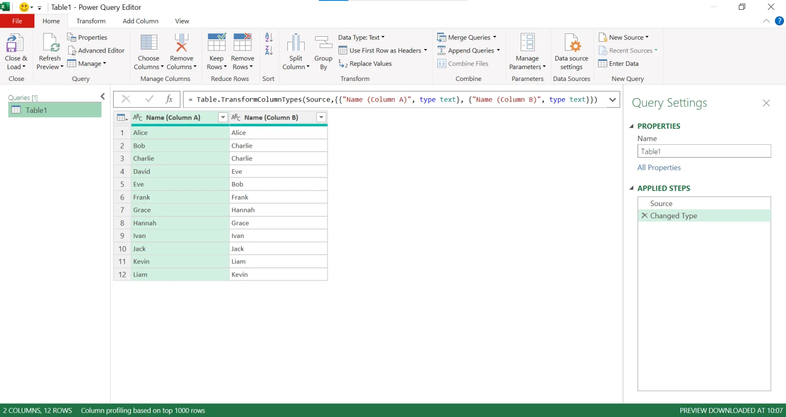
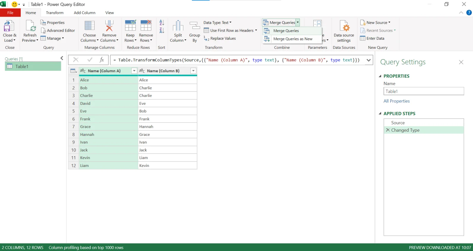
4. Use the Merge Queries option.
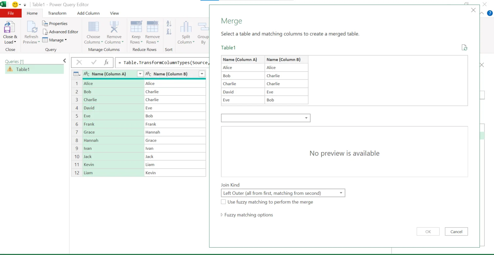
5. Choose Join type:
Power Query is recommended when working with thousands or millions of rows because it handles large data more efficiently than formulas.
One question I often get from Excel beginners is: “Which comparison method should I use?” The truth is that there is no single method that works best in every situation. Over the years, I have used different comparison techniques depending on the size of the dataset, the type of analysis required, and the version of Excel available. Choosing the right method can save a lot of time and help you avoid unnecessary complexity.
Whenever I need to compare two columns, I first identify the goal of the comparison. Am I simply checking whether two cells match? Looking for duplicate values? Finding missing records? Or working with a large dataset containing thousands of rows? The answer usually determines which Excel feature I choose.
| Your Goal | Recommended Method | Why I Recommend It |
| Quick row-by-row comparison | Equals Operator (=A2=B2) | Fastest and easiest method for checking whether corresponding cells contain the same value. |
| Create easy-to-read results | IF() Function | Displays clear outputs such as “Match” or “Not Match,” making reports easier to understand. |
| Perform case-sensitive comparisons | EXACT() Function | Useful when uppercase and lowercase letters must be treated differently. |
| Find values that exist in another column | XLOOKUP() or VLOOKUP() | Ideal when the lists are not aligned row by row and you need to search for matches. |
| Identify duplicate values | COUNTIF() or MATCH() | Quickly detects repeated records between two columns. |
| Visually highlight matches or differences | Conditional Formatting | Excellent for audits and reviews because results are instantly visible. |
| Extract unmatched records | FILTER() Function | Creates a separate list of missing values without manually reviewing the dataset. |
| Compare thousands of rows efficiently | Power Query | Handles large datasets much better than formulas and is easier to maintain over time. |
Personally, when I am working with small datasets, I usually start with the IF() function or Conditional Formatting because they are simple and provide immediate feedback. For larger datasets, I prefer XLOOKUP or Power Query because they are more scalable and reduce the chances of manual errors. If I only need a quick answer, the equals operator remains one of the fastest tools available.
My advice is to begin with the simplest method that solves your problem. As your Excel skills improve and your datasets become larger, you can gradually move to more advanced tools such as XLOOKUP, FILTER, and Power Query. This approach keeps your spreadsheets easier to understand while still delivering accurate results.
When I was a beginner like you and started comparing two columns in Excel. I thought I could do it easily, but I missed matches and made small mistakes, which taught me how common errors can affect the final results. Following are some of the common mistakes that I want you to avoid:
1. Different data formats: Values may look the same, but differences in text, numbers or dates can cause wrong results.
2. Extra spaces in cells: Hidden spaces before or after values often lead to missed matches.
3. Using the wrong formula: Choosing an incorrect formula can show false matches or errors.
4. Case sensitivity issues: Excel treats uppercase and lowercase text differently in some functions.
5. Not checking for duplicates: Duplicate values can confuse comparisons and lead to inaccurate conclusions.
Read Also: Excel Formulas Everyone Needs to Know
I have seen many people who jump straight into formulas, and then they get confused by the results later. If you clearly understand your goal and prepare your data properly, comparing columns becomes easy. Here are some key things that you need to know before you start comparing Excel columns:
Even when the data looks the same, Excel may not read it the same way. Small differences like formatting or spacing can cause problems when you compare columns. The following are some key aspects that you should always remember:
For cleaning and standardizing data before comparison, you can use tools like TRIM or VALUE.
Every column comparison does not follow the same structure. In some cases, values must be compared row by row, while in others, the position of the data does not matter. There are two primary scenarios:
Duplicate entries can affect the reliability of comparison results, especially when using lookup functions that return only the first match. When you start comparing, always make sure that:
Comparing two columns in Excel doesn’t have to be confusing or time-consuming. In this article, you explored multiple ways to compare data from simple formulas to built-in Excel tools. Each method helps you in spotting matches, differences, duplicates, or missing values. All this, more accurately and with less effort. All the methods that are explained here follow standard Excel practices and are aligned with Microsoft’s recommended approach to data comparison and validation.
Now, your next step has to be practice. Try these methods on real files, even small ones. As your data grows, try to choose smarter techniques instead of manual checks. Over time, you will not only save hours but also avoid costly mistakes. Mastering this skill makes your Excel work cleaner, faster, and far more reliable.
Comparing two columns helps you quickly check if the data is the same or different. It makes it easy to find duplicate values, missing entries or matching data between two lists.
The one-time purchase version of Excel (such as Office 2021 or Office 2024) is bought once and does not receive major feature updates. Microsoft 365 is subscription-based and receives regular updates, new functions like XLOOKUP and dynamic array formulas, and security improvements automatically.
To compare two columns in Excel without using formulas, you can use Conditional Formatting. It highlights matching or different values automatically.
Microsoft 365 is the latest version. It is a subscription-based version that gets regular updates, new features and security improvements automatically.
Yes, COUNTIF is best for beginners. It is easy to learn and does not require complex formulas.
This happens because Excel stores values with hidden differences like extra spaces, non-breaking spaces or different data types (text vs number) even if they look identical.


Top Desktop Support Engineer Interview Questions and Answers
June 27th, 2026