Are you an Excel user struggling to search data manually? Well, it is a common issue for beginners. I have seen people scrolling through hundreds of rows just to find one value. It feels frustrating and it slows your productivity and efficiency. This is because they do not know about the VLookup Function.
It is one of the most useful Excel formulas that lets users find information quickly and accurately without doing things manually. Using it can help you improve your productivity and solve all the complications. In this guide, I will explain everything from what is VLOOKUP, how it works, and how to use it step by step with the help of real examples. Let’s begin.
Learn to use VLOOKUP to find specific data in a table by searching for a value in the leftmost column and returning a corresponding value from another column.
VLOOKUP is a combination of two words: Vertical and Lookup.
So now, when you use VLOOKUP, you are telling Excel to go to this column, find the given value, and then give me something related from another column in the same row. This is what everything VLOOKUP does. For instance, imagine if you have a list of employees. You know the employee ID, and you want to find their salary. Instead of checking each row manually, you can use VLOOKUP to do it instantly.
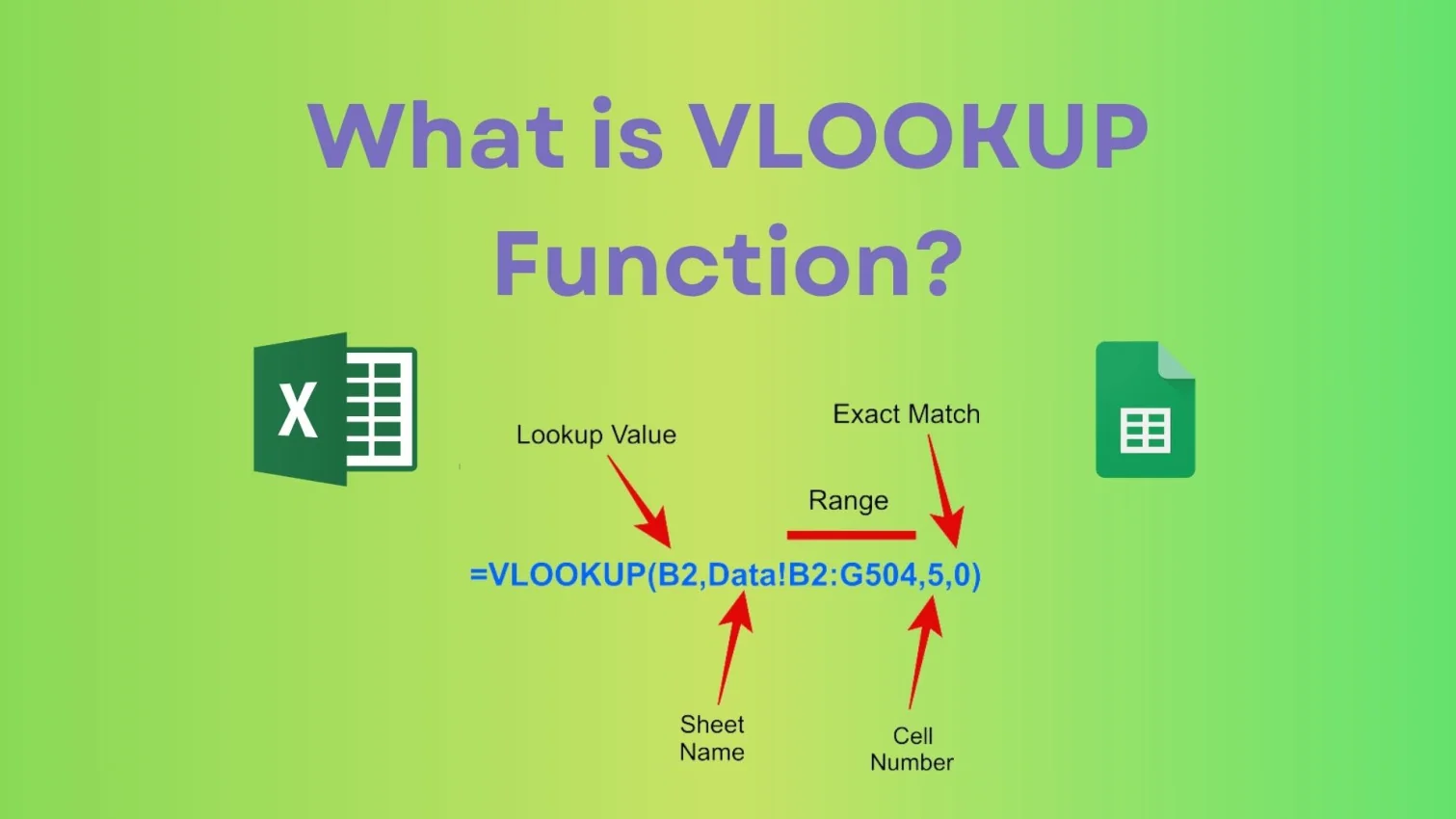
Before you start using VLOOKUP, you need to understand its structure. The formula of VLOOKUP is:
|
Let me walk you through this in a very practical way. Just follow these steps one by one.
1. Understand What You Want to Find: First, you need to be clear about one thing, that is, what exactly are you looking for? It could be an employee’s salary, a product’s price or a student’s grade. This value is called your lookup value. If you are not clear here, then the formula will not work properly.
2. Check Your Data Structure: Now look at your table carefully. The value you want to search must be in the first column of your table. This is very important because VLOOKUP always searches from left to right. If the first column does not carry your lookup, then you need to rearrange your data.
3. Select the Table Range: Next, you need to select the full table that contains your data. Do not just select one column. You need to include all the columns from the lookup column to the column where your answer exists. For instance, if your data is from A2 to C6, then your table range will be A2:C6.
4. Identify the Column Number: Now you need to tell Excel from which column it should return the result. Count the columns from left to right.
If your answer is in the third column, then you need to write 3.
5. Decide the Match Type: Now, decide how accurate your result should be, like:
In most cases, you will use FALSE because you want the exact value.
6. Write the VLOOKUP Formula: Now combine everything and start typing -
|
Then enter your lookup value, table range, column number, and match type.
For instance:
|
7. Press Enter and Check the Result: Press Enter and Excel will give you the result instantly. If everything is correct, then you will see the value you wanted. If not, check your inputs again. Most errors happen because of small mistakes like a wrong range or an incorrect column number.
Now, let’s understand this with real examples. This is where everything becomes clear.
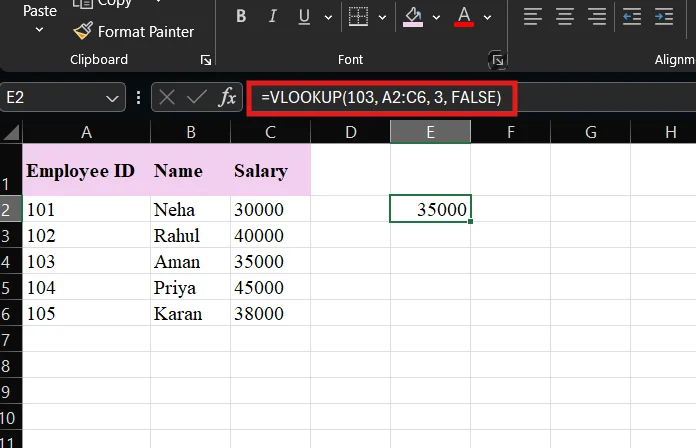
To find the salary of employee ID 103, use the given formula:
|
Output: 35000
Let’s understand what is happening here. You are asking Excel to find 103 in the first column. Then, you are telling Excel to return the value from the third column. FALSE means you want an exact match.
The result will be 35000.
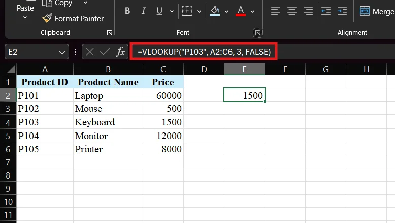
To find the price using the Product ID, use the given formula:
|
Output: 1500
Here again the same logic is used. Excel searches for P103 in the first column. Then it returns the value from the third column and the result is 1500.
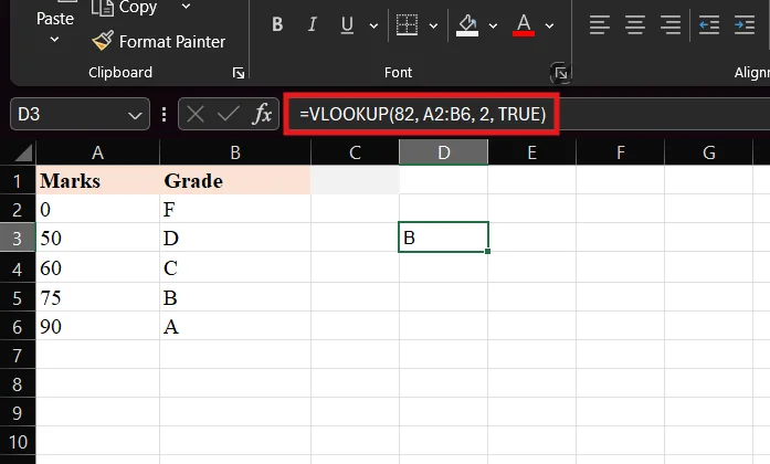
To find grade for 82:
|
Output: B
This time, in the formula I used TRUE. This means Excel will not look for an exact match. Instead, it will find the closest lower value. So, 82 is between 75 and 90. Excel has picked 75 and returns grade B. This is very useful when you are working with ranges like marks, discounts or commissions.
Before you do it practically, you need to be aware of some common mistakes. Almost everyone makes these when they start. Let’s begin.
This is the most common error. It means Excel cannot find the value. Now, why does N/A Error happen?
You can fix it by checking your data and using exact match (FALSE).
Sometimes you get the wrong answer. This usually happens when you give the wrong column number. That is why always double-check your column index.
This is a limitation of VLOOKUP. If your lookup value is not in the first column, VLOOKUP will not work. You will need to rearrange your table or you can use XLOOKUP in place of that.
If you use TRUE, your data must be sorted. If it is not sorted, Excel will give incorrect results. So you should always be careful with approximate matches.
Excel now has two main lookup functions, including VLOOKUP and XLOOKUP. XLOOKUP is more powerful than VLOOKUP. Let’s see their key differences.
| Feature | VLOOKUP | XLOOKUP |
|---|---|---|
| Lookup Direction | Works only from left to right | Works in both directions (left and right) |
| Lookup Column Requirement | Lookup value must be in the first column | No such restriction |
| Column Reference | Uses column number (like 2, 3, 4) | Uses direct column or range reference |
| Ease of Use | Slightly tricky for beginners | Easier and more intuitive |
| Error Handling | Returns #N/A if not found | Can return custom message like "Not Found" |
| Exact Match Default | Needs FALSE for exact match | Exact match is default |
| Approximate Match | Requires TRUE and sorted data | Supports approximate match without strict sorting |
| Flexibility | Limited functionality | Highly flexible |
| Performance | Slower with large data | Faster and more efficient |
| Multiple Criteria Lookup | Not directly supported | Can handle more complex lookups |
| Data Safety (Column Insert/Delete) | Breaks if columns change | Does not break easily |
| Availability | Available in older Excel versions | Available only in newer Excel versions |
You should use VLOOKUP in these types of situations:
VLOOKUP may feel a little confusing in the beginning, yet once you start using it, it will become very easy for you. It helps you in finding data quickly with you even scrolling or searching manually. You can definitely save your time, reduce errors and handle large datasets easily. Even basic knowledge of VLOOKUP can make your Excel work much smoother.
The best way to learn it is by practicing with real examples. You need to start small, try different cases and that’s how you can slowly build your confidence in excel. As you get comfortable, you can also explore advanced functions like XLOOKUP or INDEX-MATCH. Yet, when you have a strong hold on VLOOKUP, It will give you a solid foundation that will always be useful.
Yes, it is still widely used in many companies and basic Excel tasks.
It can only search from left to right and needs the lookup value in the first column.
You should use TRUE when working with ranges like marks or grading systems.
Yes, XLOOKUP is more flexible and easier, but VLOOKUP is still important to learn.