Blank rows in Excel do not seem to be a problem, but they can quietly break your workflow. I am also a data professional working with Microsoft Excel for a long time. Trust me, removing blank rows from your datasets should be one of the first things you should do before applying any function or formulas.
These empty-looking rows often hide spaces, formulas, or formatting that disrupt sorting, filtering, and calculations without warning. Do you know how to remove blank rows in Excel? Don't worry. I will explain every method, step-by-step, with examples, best practices, and the reasons why blank rows appear.
Blank rows can affect how a worksheet behaves during sorting, filtering and calculations. They may interrupt data ranges, cause formulas to stop early or make reports harder to read and maintain. Removing them helps keep your data neat, clear and manageable. Here is why removing blank rows is important:
One simple way to remove blank rows in Excel is to delete them manually. This involves selecting the empty row, right-clicking on it, and choosing the Delete option. While this method is straightforward and works for very small datasets, it quickly becomes impractical when you are working with large or frequently updated data.
That’s where more efficient and reliable methods become important. These approaches allow you to clean and organize your data without risking data loss or quality issues. In the following sections, we’ll explore multiple techniques that can handle any dataset size with ease. Most of these methods also work in Google Sheets, so you won’t need to learn separate processes for different tools.
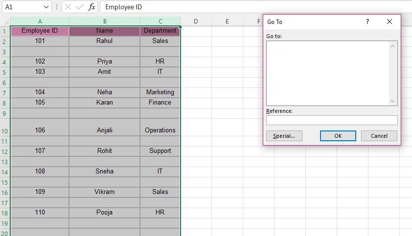
1. Select your entire data range and then press Ctrl + G or Ctrl + F5.
![]()
2. A dialogue box wgo to speacial ill appear; click on the special button.
3. Choose blanks then click OK.
![]()
4. All blank cells are selected now. Right-click and choose the delete option.
![]()
5. Select the entire row option and hit the ok button.
![]()
Your final (cleansed) data will look like this:
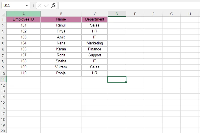
I usually use this method when I know my data is clean and does not contain formulas. It feels fast and satisfying when the blank rows are empty and easy to remove in one go. However, I have learned the hard way that Go To Special only selects truly empty cells. It does not select cells containing formulas that return empty strings (""). Because of that, I only rely on this method when I am confident there is nothing hidden in the cells.
1. Select your data, go to the “data” option from the taskbar, and click on the “create a filter” option. You can also select the filter sign appearing on the Quick Access Toolbar (QAT).
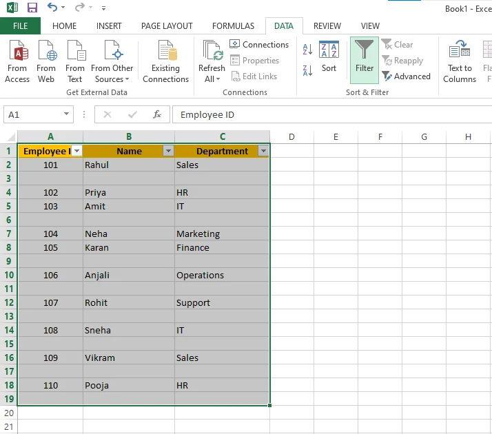
2. After that, click on any column and uncheck everything except for the blank option and hit the Ok button.
![]()
3. Now your blank rows will be visible, select them all and click on “delete selected row”.
![]()
4. Now remove the filter and your data will be free of blank rows.
This is the method I trust the most when working with important data. I like to see all the blank rows clearly before deleting them, especially in large or imported datasets. It gives me time to double-check what I am removing. The only issue I notice is that some formula-based blanks stay behind, but overall, it feels much safer than faster methods.
1. Select your whole data.
2. Go to the Sort option from the taskbar and select the A-Z option.
3. The blank rows will be placed at the end.
4. Then select the “delete” option.
![]()
5. A small box will appear, so click on the “entire row” option and select OK.
![]()
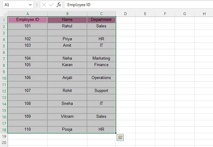
Your data will be cleansed:
I use sorting only when the order of rows does not matter to me. It helps when blank rows are scattered and hard to find manually. Once everything moves to the bottom, deleting them is easy. However, I have broken data order before by using this method carelessly. Because of that experience, I now avoid it for reports or time-based data.
1. Select your data, press Ctrl + T, ensure "My table has headers" is checked and click OK.
2. Select any column and uncheck all options except the blank option.
![]()
3. Your blank rows will be visible now.
4. Now right click and select the delete option, then go to ‘entire sheet row”.
![]()
5. Remove filters. Now you have your cleansed worksheet.
I prefer this method when I work on files that are updated regularly. Converting data into a table makes everything feel more organized and filtering blank rows becomes simpler over time. It is especially helpful for tracking data or reports. Its limitation is that Excel changes formatting automatically, which I sometimes need to adjust.
Power Query is one of the safest and most professional ways to remove blank rows in Excel. I personally prefer this method when working with large datasets or files that are updated regularly. The best part is that Power Query does not change your original data. It creates a clean version of your dataset and allows you to refresh it anytime new data is added.
1. Select your entire dataset.
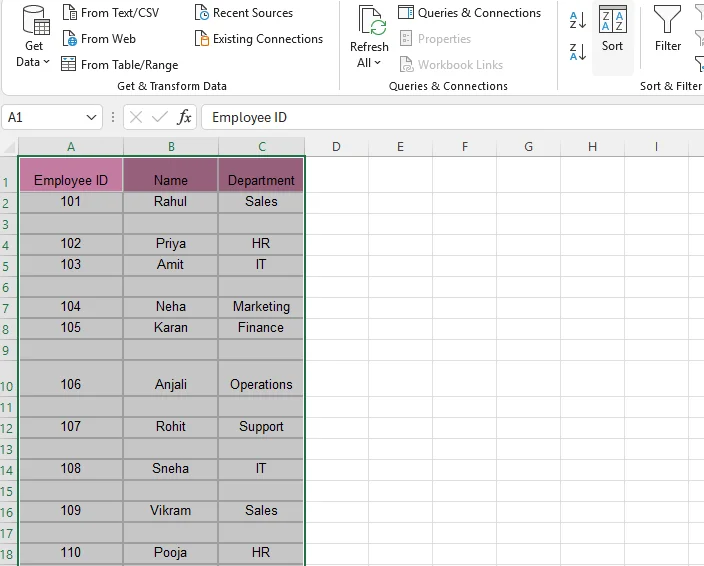
2. Go to the Data tab from the taskbar and click on From Table/Range.
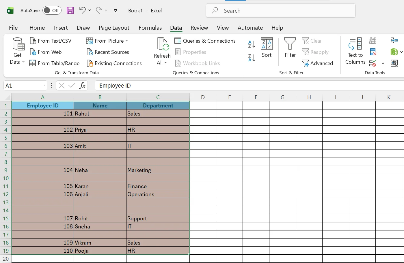
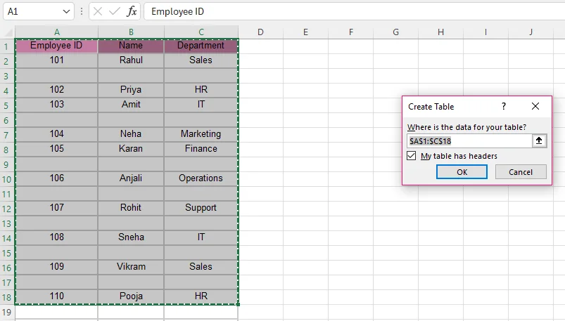
3. If your data is not already in a table format, Excel will ask you to create one. Make sure the “My table has headers” option is checked, then click OK.
![]()
4. The Power Query Editor window will open.
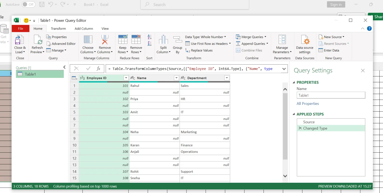
5. In the Power Query Editor, go to the Home tab and click on Remove Rows.
6. Select Remove Blank Rows.
![]()
7. Once the blank rows are removed, click on Close & Load to bring the cleaned data back into Excel.
![]()
8. Your cleaned dataset will now appear in a new worksheet without any blank rows.
![]()
I recommend this method when handling large or frequently updated datasets. It is especially useful for imported data from CSV files, databases, or external systems. Since Power Query keeps your original data untouched and allows you to refresh changes with one click, it is much safer than manual deletion. For professional reporting and data analysis, this is my most trusted approach.
If you work with Excel regularly and want to automate the process, you can use VBA (Visual Basic for Applications) to remove blank rows instantly. This method is useful when you repeatedly clean similar datasets and want to save time.
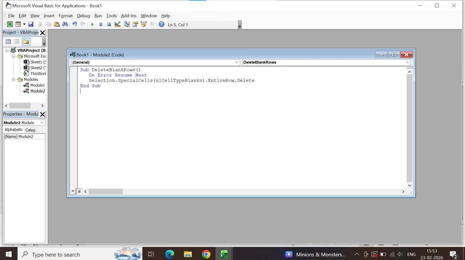
1. Press Alt + F11 to open the VBA Editor. In the top menu, click on Insert, then select Module.
![]()
2. A new module window will appear. Copy and paste the following code:
|
3. Minimize the VBA Editor, select your dataset in Excel, press Alt + F8, choose DeleteBlankRows, and click Run.
![]()
4. All blank rows within your selected range will be deleted instantly.
I use this method when I need quick automation. It works well for repetitive tasks and saves a lot of time when cleaning large datasets. However, you should always keep a backup copy of your file before running VBA code. Since macros make permanent changes, there is no easy undo option after execution. This method is best suited for advanced users or professionals who frequently work with structured data.
There are many reasons why, knowingly or unknowingly, your data can have blank rows. This usually appears when you import data without checking or editing it correctly. Excel does not clean data automatically. This means empty rows remain there unless you remove them manually. Let’s understand the common reasons for appearing blank rows:
For smaller datasets, you can easily scroll through the worksheet and identify blank rows manually. However, when working with large datasets, blank rows can be difficult to spot and may go unnoticed, creating issues during data analysis. You can refer to the following points for the same:
Read Also: 65 Best Excel Interview Questions and Answers
Before you remove blank rows in Excel, make sure you know exactly what you are doing. Small mistakes can affect your data, formulas or results, especially if the file is important. You can refer to the following practices for better understanding:
Before you start, you should always save a backup copy of your worksheet. This ensures you can restore the original data if something goes wrong.
When a cell looks empty, just click on it and check the Formula Bar. Some cells may appear blank but still contain formulas, spaces or hidden values.
Make sure your Active Cell is inside the data range before applying filters or formulas. This helps Excel work only on the selected data.
Avoid deleting rows without checking them first. Excel may not treat rows with formatting or invisible characters as truly blank.
Read Also: XLOOKUP vs VLOOKUP
In this article, I have explained why blank rows appear in Excel and how they can affect your data. I also shared five methods to remove them efficiently. After reading this, you should try these methods on your own worksheets and choose the one that works best for your data, so that you can keep your sheets clean, accurate, and organized.
Explore Our Trending Articles-
For this, you should avoid pressing Enter unnecessarily, clean imported data properly, and review formulas that return empty values instead of real blanks.
You can press Ctrl + G, then click Special → Blanks → OK. After that, right-click and delete entire rows.
You can use filters, conditional formatting or formulas to hide blank cells while keeping the data and structure of your worksheet unchanged.
Yes, Power Query is safe for large Excel datasets. It efficiently handles data transformations without altering the original files.
Yes, formulas can detect hidden blank rows. Functions like SUBTOTAL or AGGREGATE can ignore hidden rows while checking for blanks.