Are you an Excel user working on vast datasets? Well, then you may know how complicated it is to compare two ranges from the same or different datasets. In my opinion, it is one of the most frustrating tasks without using the perfect Excel formula. This is where you should consider using the XLOOKUP formula, which is also an advanced version of the VLOOKUP formula.
It can do everything that VLOOKUP does with various advanced additional functionalities. It is designed to make lookup tasks easier, faster, and more flexible. It helps you get the answer in seconds, whether you are working on small or complicated datasets. Once you understand it properly, it becomes one of those functions you will use almost every day. In this article, I will explain everything about the XLOOKUP function. Let’s begin.
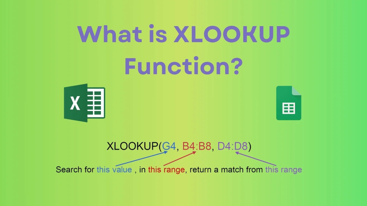
Learn how to use XLOOKUP function in Excel and Google Sheets to find a specific value by just selecting what to look for, where to look, and what to return.
XLOOKUP is a modern Excel function that allows you to search for a value in a range and return a corresponding value from another range. The biggest advantage of XLOOKUP is that it is not restricted like older functions. It works in any direction. You can look left, right, up or down.
You also do not need to count columns, which removes one of the most common errors people make with VLOOKUP. It also allows you to handle errors easily and even search from the bottom to get the latest value. XLOOKUP is considered a more powerful and user-friendly replacement or i can say a superior successor to VLOOKUP and HLOOKUP. It does not require sorted data, allows looking to the left, and defaults to an exact match.
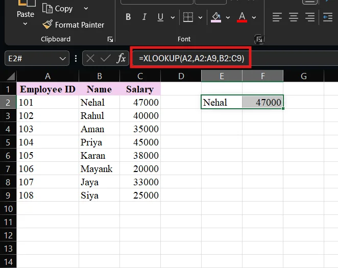
It works like this; You search for something, then Excel finds it and returns what you need. For instance, suppose you have a list of employees with their IDs and salaries. If you know the employee ID and want to find the salary, XLOOKUP will do that instantly.
To use XLOOKUP correctly, you need to understand its structure. This is the syntax of XLOOKUP:
|
Let’s make this very practical so you can apply it directly.
1. Identify what you want to search: This is your lookup value. It can be an ID, name or product.
2. Select the lookup range: This is where Excel will search for the value that you put under the lookup value.
3. Select the return range: This is the column from which you want the result.
4. Write the formula: Type the XLOOKUP formula using the correct ranges.
5. Press Enter: Excel will instantly return the result.
Also Read: Excel Cheat Sheet
Let’s look at some real examples that you can try by yourself in Excel.
If you want to find the salary of employee ID 101, you need to use:
|
Excel will search for A2 in column A and return the corresponding salary from column C with their name from column B.
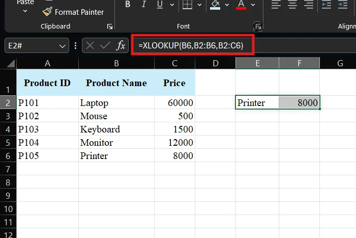
If you want to find the price of B6, use:
|
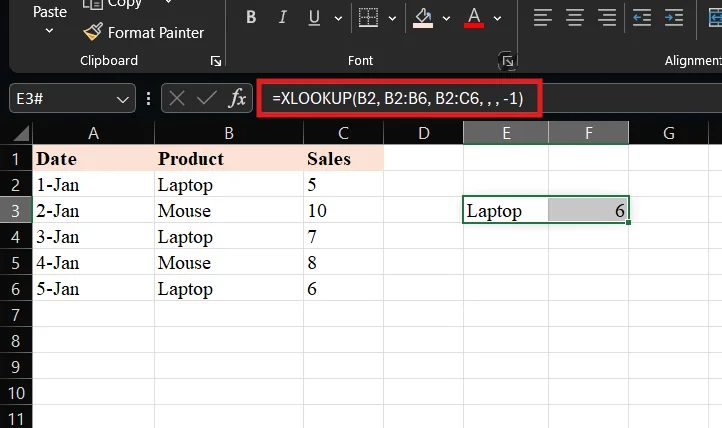
If you want the latest sales value of “Laptop(as in B2 is laptop)”, use:
|
Even though XLOOKUP is simple, you may still face a few common issues.
This happens when the value is not found in the lookup range. You can fix it by adding a custom message:
|
Sometimes the formula runs, but the result is wrong. This usually happens because of extra spaces or mismatched data. You can fix this by cleaning your data or using TRIM.
If numbers are stored as text, XLOOKUP may not match them correctly. Make sure your data types are consistent.
If your lookup array and return array are not aligned properly, the result will be incorrect. Always ensure both ranges have the same size.
Both XLOOKUP and VLOOKUP are used to find and return data in Excel, but XLOOKUP is more flexible and easier to use. Here’s a quick comparison for you to understand the key differences:
| Feature | XLOOKUP | VLOOKUP |
|---|---|---|
| Direction | It can work in any direction (left, right, up, down) | It only works left to right |
| Column Reference | No need to count columns | It requires a column index number |
| Error Handling | Built-in (if_not_found) | Needs IFERROR separately |
| Default Match | It is an exact match by default | It is an approximate match by default (can cause errors) |
| Search Mode | It can search from the top or the bottom | It only searches from the top |
| Handling Missing Values | It can return a custom message | It shows #N/A error |
| Flexibility | It is very flexible | It has limited flexibility |
| Ease of Use | It is simple and readable | It is slightly confusing for beginners |
| Performance | It is better for large datasets | It is slower with large data |
| Availability | Excel 365, Excel 2021 | It is available in older versions of Excel. |
You should use XLOOKUP in almost all modern Excel tasks. It is especially useful when:
XLOOKUP is one of the most powerful and practical functions in Excel. It simplifies the process of finding and retrieving data. This makes your work faster and cleaner. If you take a little time to practice it, then you will notice a big difference in how you work with Excel.
Tasks that used to feel confusing will start feeling simple. Once you get comfortable with XLOOKUP, you will naturally prefer it over older functions because of its flexibility and ease of use.
Yes, XLOOKUP is more flexible, easier to use, and removes many limitations of VLOOKUP.
No, it is available in Excel 365 and Excel 2021.
Yes, XLOOKUP can work with both text and numbers.
If the values are not found, then it shows #N/A. Yet, you can always replace it with a custom message.
No, it is simple to learn XLOOKUP. Once you understand the basics, you can use it easily in real work.