Microsoft Excel is not just an ordinary tool. It has been a go-to solution for managing data with different features like formulas and functions, pivot tables, charts and graphs, data validation, conditional formatting and macros (VBA). Excel is used by hundreds of millions of professionals worldwide and building a career with this tool can really be rewarding.
Are you preparing for such a job? Consider this comprehensive list of the most asked Microsoft Excel interview questions and answers, focused on testing your ability to work with formulas, functions, PivotTables, data analysis tools and real-world business scenarios.
Let's begin with the most basic Excel interview questions and answers. These are designed for beginner-level candidates.
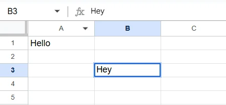
The cell address is the location of a cell into a spreadsheet. Think of it as a general location that includes the latitude and longitude. Here, the latitude and longitudes are the row and column numbers. For instance, if a cell is present in the 3rd row and 2nd column, the address would be B3, where B stands for the column and 3 stands for the row.
The ribbon is the bar you see at the top of your Excel sheet. It includes various buttons like Home, Edit, Insert, etc., and icons like bold, filter, etc. It is one of the best functions of Excel, which gives access to different features on a click. For instance, you want to filter data or include a hyperlink, just use their icons. You can also customize the ribbon according to your preference.

Data validation is a special option that allows users to restrict a range of cells on what value it will take. It comes under the Data Tools group of the Data tab. For instance, if you apply List Data Validation to a column, you can define a specific list of names that are allowed.
Attempting to enter any value not on that list, or even a different data type if the list contains only text, will throw an error. Similarly, you could restrict a column to only accept whole numbers within a specific range.
Both SUBSTITUTE and REPLACE functions modify text strings, but they differ in how they identify the text to be replaced. SUBSTITUTE replaces specific text strings, while REPLACE replaces text based on its position within the string. Let's take an example of a string 'happy77' in A1 cell. The use of these functions will be as follows:
Macros is a programming concept based on the Visual Basic for Applications (VBA) programming language. Recording macros does not require programming knowledge, but editing or customizing macros requires basic VBA understanding. It is a feature that allows users to automate a certain series of tasks. To use it first, you have to record the series of tasks and then execute all of them in the same way with just one click.
There were two types of macro languages used on this platform, including VBA and XLM. VBA is the most used one in the latest Excel versions. VBA is the standard, while XLM macros are deprecated and often disabled for security reasons. While XLM was popular in the old versions.
Microsoft Excel has over 500 built-in functions as of 2026. These functions cover mathematical, statistical, logical, text, date & time, lookup, and many other categories. While there are hundreds of functions, most professionals regularly use only 50–100 core ones.
There are two ways to freeze panes. You can select the cell below the rows and to the right of the columns that you want to freeze, then navigate to the View tab and click on Freeze Panes. Alternatively, you can freeze the top row or the first column, specifically using the other options in the dropdown.
To create a simple chart, first select the data you want to add in the chart. Then, navigate to the insert tab and choose the chart type you want to use.
Workbook in the entire file with the .xlsx extension where you are working. A worksheet is the sheet you create within a workbook. A single workbook can contain multiple worksheets that appear at the bottom of it.
Cell references control how a formula behaves when copied to another cell.
To toggle between reference types, select the cell reference in the formula bar and press F4.
All four are counting functions, but they count different things:
Conditional Formatting automatically applies visual formatting, such as colours, icons, or data bars, to cells based on rules or conditions you define. It helps users instantly spot trends, outliers, and patterns in data without writing formulas.
For example, you can highlight all sales figures below a target in red, or use a colour scale to show performance from lowest (red) to highest (green) across a dataset. To apply it, select the range, go to Home > Conditional Formatting, and choose a rule type. You can create custom rules using formulas for more advanced use cases.
It is commonly asked in interviews because it tests a candidate's ability to make data visually meaningful, a core skill for reporting and dashboards.
Now, we will discuss the most asked intermediate-level Excel interview questions and answers. It is most beneficial for individuals who want to change their company or boost their career.
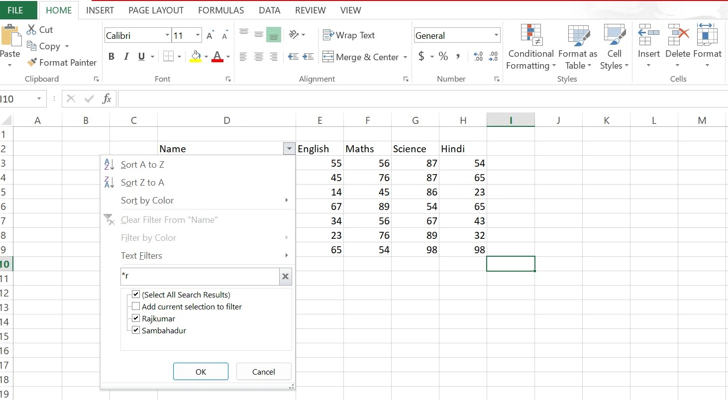
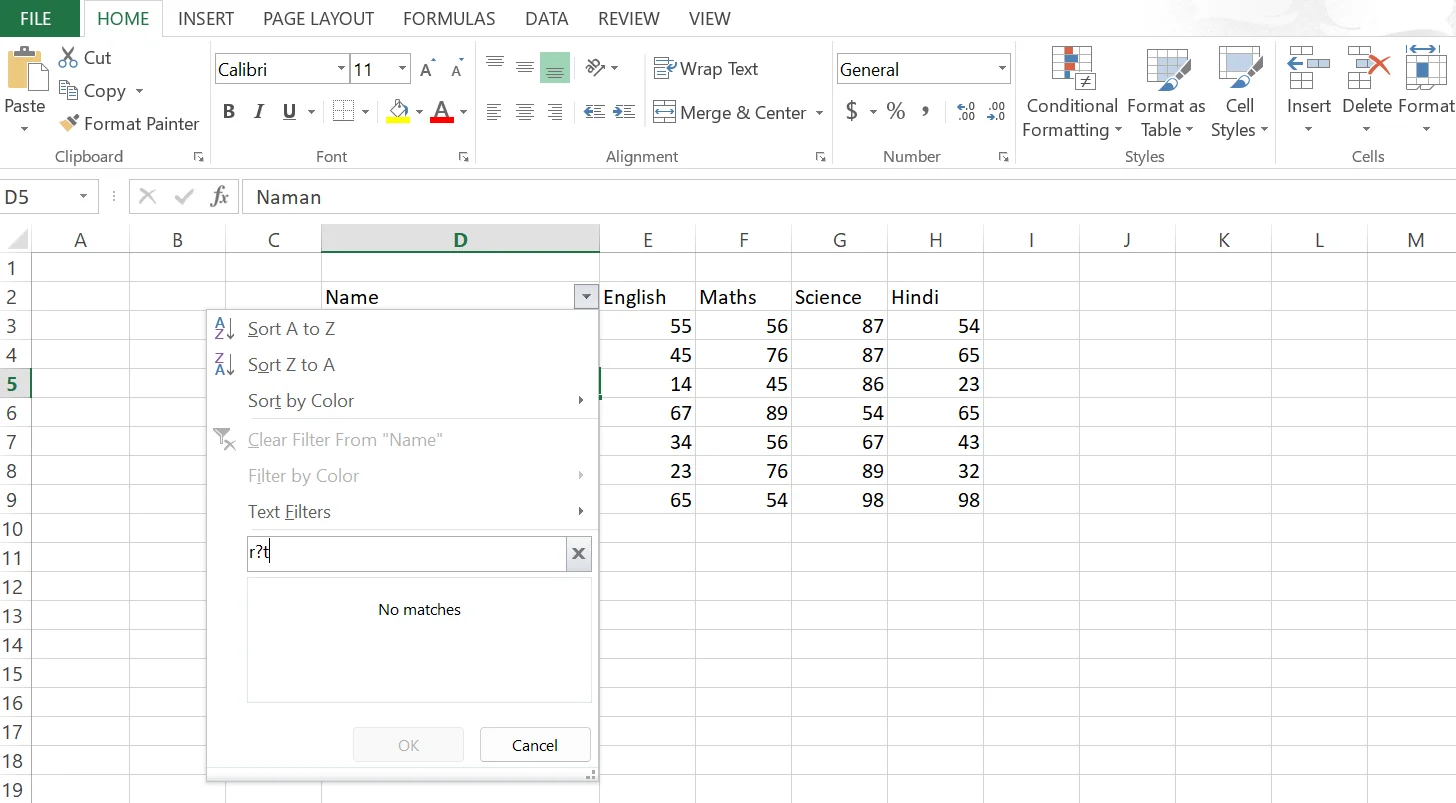
Wildcards are unique characters used to replace characters from a text string while filtering, searching, or using formulas for estimated matches. They help to detect data based on different patterns rather than exact matches. Here are some of their example:
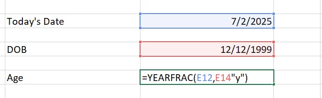
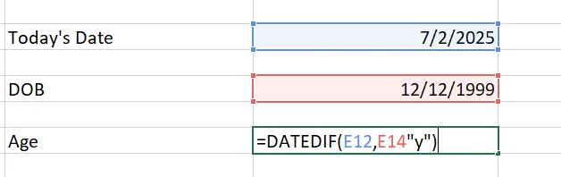
There are primarily two functions for date differences:
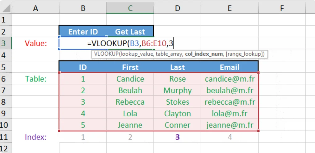
VLOOKUP or Vertical Lookup is a powerful function for retrieving data from tables based on a matching value. It searches for a specific value from a particular column (lookup column) and then returns the corresponding value from another column but the same row.
Note: In modern Excel interviews, candidates are expected to understand XLOOKUP, which is more flexible and reliable than VLOOKUP.
Important Note for 2026: In modern interviews, recruiters expect you to know XLOOKUP, which is more flexible and safer than VLOOKUP. Many companies now prefer XLOOKUP over VLOOKUP and INDEX-MATCH.
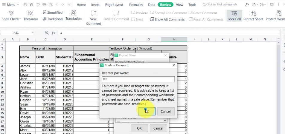
Restricting a cell from being copied involves the following steps:
Both of them are used to perform different operations but in distinct approaches. The formulas are user-defined, meaning the user can perform any action by creating formulas based on specific rules. The functions are in-built formulas that come with a specific syntax and purpose. It provides efficiency in performing common tasks, whereas the formulas provide flexibility.
A pivot table summarizes data in a structured way that helps users analyze and understand humongous datasets. It also enables them to quickly calculate, categorize and filter insights from a spreadsheet. PivotTables are also the foundation for building interactive Excel dashboards. This allows them to uncover different perspectives on the available data. Creating a pivot table involves the following steps:
The IFERROR function is mostly used to manage the errors in formulas. It sets formulas to return a specified value instead of the default error message. It is particularly useful when you want to avoid displaying error messages like #DIV/0!, #N/A, or #VALUE! to the user or want to provide a more user-friendly output.
The COUNTIF function counts cells within a range that meet a single specified criterion, while COUNTIFS allows for counting cells that meet multiple criteria across one or more ranges. Essentially, COUNTIF handles single conditions and COUNTIFS handles multiple conditions, making it more versatile for complex counting tasks.
Array formulas are the best way to perform calculations on multiple cells simultaneously. They can handle multiple calculations within a single cell or return multiple results. This offers a more efficient way to manage complex tasks than standard formulas. These are mostly used when the user wants to apply the same logic for the entire row or column.
Note: In modern Excel (365), Dynamic Arrays replace traditional array formulas and do not require Ctrl+Shift+Enter.
Named Ranges are used to assign names to ranges or cell references. Creating it involves the following steps:
It is quite easy to merge datasets using Power Query. You just have to navigate the Data > Get Data > Combine Queries > and Merge. This will show you a dialogue box. Here select the datasets and their common columns that have to be merged.
Once you load the data, use the transformation tools of Power Query to clean or transform it. For instance, you can split columns, filter rows or even change data types. This will help you ensure consistency of the merged dataset.
If you want to explore data transformation in more depth, Power Query in Excel is worth learning.
The Data Analysis Toolpak is an Excel feature that includes various tools for performing complicated statistical and engineering analyses. It allows users to quickly calculate and display results in output tables and generate charts. This saves time and effort compared to manually calculating the same results using formulas. To use it:
1. Enable the add-in: Go to File > Options > Add-Ins > Select Excel Add-ins in the Manage dropdown and click Go > Check the box next to Analysis ToolPak and click OK.
2. Access the tools: Navigate to the Data tab on the Excel ribbon > and In the Analysis section, click Data Analysis to view the available tools.
3. Choose a tool: Select the desired analysis tool from the list (e.g., t-test, regression, ANOVA).
4. Input data and parameters: Specify the input data range and any required parameters for the chosen analysis.
5. View results: The Toolpak will generate an output table with the results of the analysis, and potentially a chart as well, depending on the chosen tool.
There are two ways to work on both of these platforms together. You can import an Excel workbook to Power Bi or directly connect to the semantic model of Excel. The choice depends on requirements and preference. Importing involves loading the Excel data into Power BI, whereas connecting allows analyzing existing Power BI datasets directly within Excel.
Excel 365 Copilot can be used to automate tasks through AI. It helps to understand natural language prompts and build or customize Excel content. It can create new columns with formulas, add visualizations like PivotTables and charts to highlight data based on criteria and can suggest formulas, build PivotTables, create summaries, and assist with automation, though VBA code still requires manual review.
The RANK function or its equivalents like RANK.EQ and RANK.AVG are used to calculate the rank of a value in an Excel dataset. It determines the numerical rank of a given number within a specified range of numbers that indicates its position relative to other values.
To combine data from different sheets, I would use VLOOKUP or XLOOKUP to fetch matching values based on a common key. For example, if Sheet1 has employee IDs and Sheet2 has employee names, I would use:
=VLOOKUP(A2, Sheet2!A:B, 2, FALSE)
=XLOOKUP(A2, Sheet2!A:A, Sheet2!B:B)
This pulls the matching name into Sheet1 based on the employee ID. VLOOKUP requires FALSE for exact matches, whereas XLOOKUP uses exact match by default.
ActiveWorkbook and ThisWorkbook are different in the following aspects:
| Feature | ActiveWorkbook | ThisWorkbook |
| Definition | Refers to the workbook currently active (in focus) | Refers to the workbook where the code is written |
| Context Sensitivity | Can refer to any open workbook that is currently active | Always refers to the specific workbook containing the code |
| Changes if User Switches Workbook? | Yes | No |
| Typical Use Case | Used when working with the user's currently open/active workbook | Used when modifying or referencing the workbook with the macro |
| Risk of Error | Higher: if the wrong workbook is active, the macro might affect the wrong file | Lower: always acts on the correct workbook |
| Example Usage | ActiveWorkbook.Save | ThisWorkbook.Save |
There are various methods to find the last row of a column in VBA. I prefer to use the most common End(xlUp) method. This works like pressing Ctrl + upwards arrow from the bottom of the worksheet.
Dim lastRow As Long lastRow = Cells(Rows.Count, "A").End(xlUp).Row ' Finds last row in Column A |
You can easily calculate the area of a rectangle in VBA by creating a custom function. Here is a simple example:
Function RectangleArea(length As Double, width As Double) As Double RectangleArea = length * width End Function |
The OpenDocument format is a robust extension (.ods) in Excel. It stands for OpenDocument Spreadsheet, used for storing spreadsheet data. ODF is designed to provide a vendor-neutral, open standard for office applications. This makes it compatible with various software, including LibreOffice, Apache OpenOffice and more.
Both functions add up values based on conditions, but they differ in how many conditions they support.
Key rule: in SUMIFS, the sum_range always comes first, whereas in SUMIF it comes last. This is a common mistake candidates make in interviews.
Both functions combine text from multiple cells, but TEXTJOIN is significantly more powerful for modern Excel.
TEXTJOIN is especially useful when combining data across a range, something CONCATENATE cannot do without referencing each cell individually.
Both are lookup functions but they search in different directions:
In practice, most business data is column-oriented, making VLOOKUP far more common. In modern Excel interviews, both are largely superseded by XLOOKUP, which handles both vertical and horizontal lookups in a single flexible function.
This section includes the most asked advanced-level Excel interview questions and answers. It includes the advanced-level concepts and experience-based questions to help experienced professionals in cracking their next interview.
Use of INDEX-MATCH over VLOOKUP() offers various advantages, including:
However, in 2026, XLOOKUP is often recommended as it combines the best of both with simpler syntax and better error handling.
To create a dropdown list using data validation in a spreadsheet, you need to follow the given steps:
Let's take an email address as instance@igmguru.com in cell A1. You have to enter the given formula in any other cell and it will automatically yield igmguru.com.
=RIGHT(A1, LEN(A1) - FIND("@", A1)) |
Yes, it is possible to apply a filter on data using Slicer. Start with ensuring that your data is organized in a proper way or is a part of the Pivot Table. Next, click on the table, navigate the Insert tab and click on the Slicer.
You will see a dialog box on your screen, check the boxes of columns where you want to apply the slicer and then click ok. Now you will see the slicer on your worksheet. Use it to filter your data by simply clicking the options it gives.
There are several methods to effectively manage missing data in Excel. These include detecting the missing values, deleting or replacing them with appropriate ones and using the built-in functions of Excel for data manipulation. Methods for handling missing data range from simple deletion to more complex imputation techniques.
For instance, in a new column, you could use a formula like =IF(ISBLANK(A2), AVERAGE($A$2:$A$100), A2). When this formula is dragged down, it will replace blank cells in column A with the average of the non-blank values in the original range A2:A100, while keeping existing values." (This is a subtle but important distinction for how imputation is often practically done).
We can use the PERCENTILE.EXC() or PERCENTILE.INC() functions to calculate percentiles. For instance, =PERCENTILE.INC(A1:A100, 0.75) can calculate the 75th percentile of the cell A1:A100 in a given dataset. Similarly, use the =QUARTILE(A1:A100, 1) for the first quartile to find its quartiles.
The CUBEVALUE function retrieves aggregated values from a dataset connected to Excel Data Model or OLAP cube. It is used to dynamically pull data based on specified criteria that provides a flexible way to interact with your data model. Essentially, it combines CUBEMEMBER functions to define the context and then extracts the relevant value.
Structured references help to refer to any elements of the Excel Table by their name rather than cell. Here are some of their syntaxes:
Creating a forecast sheet in Excel involves the following steps:
What-If Analysis is a robust feature that helps users to explore different scenarios by modifying input values in a spreadsheet. It allows them to observe the impact on results of formulas and calculations. This approach provides a better understanding of how variations in assumptions affect outcomes, aiding in decision-making and strategic planning.
Data analyst roles test a specific subset of Excel skills, focused on data cleaning, aggregation, lookup functions, and producing analysis-ready outputs. These are the most commonly asked Excel interview questions in data analyst interviews across companies like TCS, Infosys, Amazon, and Accenture.
Cleaning a dataset typically involves several steps. First, I remove duplicate rows using Data > Remove Duplicates or the UNIQUE function. Then I handle inconsistent text using TRIM (removes extra spaces), PROPER or UPPER (standardises case), and SUBSTITUTE (removes unwanted characters). For missing values, I use filters or ISBLANK() to identify blanks and decide whether to delete, fill, or flag them. Finally, I check data types, ensuring dates are formatted as dates and numbers aren't stored as text, using the Text to Columns tool or VALUE() function to convert where needed. Power Query is the most efficient tool for repeatable cleaning workflows on large datasets.
PivotTables are the fastest way to summarise and explore large datasets without writing formulas. I use them to aggregate data by category (e.g., total sales by region), identify trends over time, compare segments, and surface outliers. For analysis, I drag dimensions like Date or Region into Rows, metrics like Revenue into Values, and use slicers for interactive filtering. I always convert the source data into an Excel Table first (Ctrl+T) so the PivotTable automatically captures new rows when refreshed. For more dynamic analysis, I combine PivotTables with calculated fields and the GETPIVOTDATA function to pull specific values into summary reports.
All three are conditional aggregation functions that operate on a range meeting a specified criterion:
For multiple conditions, use COUNTIFS, SUMIFS, and AVERAGEIFS, respectively.
I identify outliers using statistical thresholds. The most common approach is the IQR (Interquartile Range) method: calculate Q1 using =QUARTILE(range,1) and Q3 using =QUARTILE(range,3), then compute IQR = Q3 - Q1. Any value below Q1 - 1.5*IQR or above Q3 + 1.5*IQR is flagged as an outlier. I then use a helper column with an IF formula to label these rows and filter or exclude them. For visual identification, a Box and Whisker chart in Excel quickly shows the distribution and flags outliers without manual calculation.
Power Query is the preferred tool for repeatable, scalable data preparation. I use it to: import data from multiple sources (CSV, SQL, SharePoint, web), merge and append datasets using common keys, unpivot columns to reshape data for analysis, remove duplicates and errors, and apply transformations like splitting columns, changing data types, and filtering rows. The key advantage is that the entire transformation is recorded as steps, so when new data comes in, I simply refresh the query and all cleaning and shaping happens automatically without re-doing manual work.
The core functions a data analyst is expected to know confidently are: XLOOKUP / INDEX-MATCH (data retrieval), SUMIFS / COUNTIFS / AVERAGEIFS (conditional aggregation), IF / IFS / IFERROR (logic and error handling), TEXT / TRIM / CONCATENATE / TEXTJOIN (text manipulation), SORT / FILTER / UNIQUE (Dynamic Array functions for analysis), PIVOT TABLES (summarisation), and Power Query (data transformation). In 2026, knowledge of LAMBDA and LET for custom reusable functions is increasingly valued in senior analyst roles.
Dynamic Arrays are a modern Excel feature that allows formulas to return multiple values automatically into adjacent cells. Instead of copying formulas down manually, the result “spills” into nearby cells. This fundamentally changes how formulas behave in Excel 365. This makes calculations faster, cleaner, and less error-prone. Functions like FILTER, SORT, and UNIQUE are built specifically for Dynamic Arrays.
The #SPILL! error occurs when a Dynamic Array formula cannot display its results because something is blocking the spill range. Common causes include existing data in adjacent cells, merged cells or insufficient space. To fix it, clear the blocking cells, unmerge cells or move the formula to an empty area where Excel has enough space to display the results.
XLOOKUP is a modern replacement for both VLOOKUP and INDEX-MATCH. Unlike INDEX-MATCH, XLOOKUP uses a single function, supports left-to-right and right-to-left lookups, handles errors gracefully and does not break when columns are inserted. While INDEX-MATCH is still powerful and widely supported, XLOOKUP is simpler, more readable, and preferred in modern Excel interviews.
The FILTER function extracts data from a range based on specified conditions and returns only the matching records. It is widely used in data analysis, reporting and dashboards to create dynamic views without helper columns or PivotTables. FILTER is especially useful when analysts want live, formula-driven tables that update automatically as source data changes.
The UNIQUE function returns a list of distinct values from a dataset. It is commonly used to remove duplicates, generate category lists or prepare summary reports. In data analysis, UNIQUE eliminates the need for advanced filters or manual deduplication, making it easier to analyze customers, products, regions, or any repeating values dynamically.
SORT arranges data based on its own values, either in ascending or descending order. SORTBY, on the other hand, sorts one range based on the values of another range. SORTBY is more flexible and is often used when sorting names by sales, dates by priority, or any scenario where the sort logic depends on a different column.
The LET function allows users to assign names to intermediate calculations within a formula. This reduces repeated calculations, improves performance and makes complex formulas easier to read and maintain. LET is especially important in large workbooks where the same logic is used multiple times, helping improve both efficiency and clarity.
The LAMBDA function allows users to create custom reusable functions without using VBA. It enables advanced users to encapsulate complex logic into a single function that can be reused across the workbook. LAMBDA is used when repetitive calculations occur frequently and consistency, maintainability and reusability are required.
Dynamic Arrays allow dashboards to update automatically without manual range adjustments. Charts, PivotTables, and formulas can reference spilled ranges, ensuring dashboards stay accurate as data grows. This reduces maintenance effort and makes dashboards more scalable, especially when working with frequently changing datasets.
Excel 365 includes Dynamic Arrays, XLOOKUP, LET, LAMBDA, Power Query enhancements and AI features like Copilot, which are not available in older versions. These features allow analysts to work faster, reduce formula complexity and handle larger datasets efficiently. As a result, Excel 365 is now the preferred version in modern analytics and business environments.
Python in Excel allows you to run Python code directly inside Excel cells using the =PY function. It combines the ease of Excel with the power of Python libraries (pandas, matplotlib, seaborn, etc.) for advanced data cleaning, statistical analysis, and machine learning tasks without leaving the spreadsheet. Use it when you need more advanced analysis than traditional formulas can handle.
Microsoft 365 Copilot in Excel uses natural language to help users create formulas, build charts, clean data, generate summaries, and even create full dashboards. You can type prompts like “Create a sales trend chart” or “Explain this formula.” In 2026, Copilot also supports Python integration and step-by-step reasoning, making it a game-changer for productivity.
Finance analyst, investment banking, and FP&A roles test Excel at a deeper level, focused on financial functions, modelling best practices, and scenario analysis. These Excel interview questions are specifically asked in finance-focused interviews.
The most important financial functions tested in interviews are:
Sensitivity analysis tests how changes in key inputs affect an output like profit or NPV. In Excel, the best tool for this is a Data Table (under What-If Analysis). For a one-variable sensitivity, I set up the input variable in a column, link the output formula to the top-left cell of the table, and use Data > What-If Analysis > Data Table. For a two-variable sensitivity (e.g., price vs. volume), I arrange one variable in a row, another in a column, and run a two-input data table. This produces a matrix of outcomes, often colour-coded with Conditional Formatting to show the range of results at a glance.
Both metrics evaluate investment viability but from different angles. NPV gives you the absolute value added by an investment in today's dollars, a positive NPV means the investment creates value above the required return rate. IRR gives you the percentage return of the investment, which you compare against a hurdle rate. Use NPV when comparing mutually exclusive projects of different sizes, it tells you which creates more absolute value. Use IRR when communicating to stakeholders who prefer percentage returns or when comparing against a fixed cost of capital. Important caveat: IRR can be misleading for projects with non-conventional cash flows (multiple sign changes), where NPV is more reliable.
Goal Seek is a What-If Analysis tool that works backwards, you specify the desired output and Excel calculates the required input. In financial modelling, I use it to answer questions like "What sales volume do we need to break even?" or "What interest rate makes this investment viable?" To use it: go to Data > What-If Analysis > Goal Seek, set the cell containing the output formula, enter the target value, and specify which input cell Excel should adjust. Goal Seek solves for a single variable, for multi-variable optimisation, Excel Solver is the appropriate tool.
A loan amortisation schedule breaks each payment into its interest and principal components over the loan term. I build it using these steps: set up inputs (loan amount, annual interest rate, term in months), calculate the monthly payment using =PMT(rate/12, term, -loan_amount), then for each period calculate: Interest = Opening Balance × Monthly Rate, Principal = Payment - Interest, Closing Balance = Opening Balance - Principal. The IPMT and PPMT functions can also directly calculate the interest and principal portions of any specific payment. This is a common practical exercise in finance interviews, candidates are often asked to build one from scratch.
Modern Excel interviews often include scenario-based questions to test how candidates solve real business problems using formulas, PivotTables, Power Query, dashboards, and automation features. These questions help interviewers evaluate practical thinking, analytical ability, and efficiency in handling large datasets.
I would first use Conditional Formatting with the “Duplicate Values” option to quickly highlight repeated records. For advanced analysis, I could use COUNTIF or UNIQUE functions to identify duplicates dynamically. In large business datasets, Power Query can also be used to remove duplicates efficiently while preparing clean data for reporting or analysis.
I would automate the workflow using Power Query, PivotTables, and Excel formulas. Power Query can automatically clean and merge incoming datasets, while PivotTables and charts can refresh dynamically. If repetitive actions are involved, I may also use VBA macros for automation. This reduces manual effort, minimizes errors, and improves reporting speed.
I would first identify missing values using filters, Conditional Formatting, or functions like ISBLANK(). Depending on the business requirement, I could remove incomplete rows, replace blanks with default values, use averages for numerical data, or fill missing categories appropriately. The approach depends on whether the missing data affects reporting accuracy or business decisions.
I would use Excel Tables, PivotTables, slicers, charts, and Dynamic Arrays to create a scalable dashboard. Converting raw data into Excel Tables allows automatic range expansion whenever new data is added. I would then connect PivotTables and charts to slicers for interactivity. Power Query can also be used if the data comes from multiple external sources.
The most efficient approach is using Power Query because it can merge and transform multiple worksheets automatically. For smaller datasets, functions like VLOOKUP, XLOOKUP, INDEX-MATCH, or FILTER can also combine information based on common fields such as employee IDs, product IDs, or dates. Power Query is generally preferred for scalability and automation.
I would start by ensuring the data is in an Excel Table for easy range management. I would then use the LARGE function or sort the dataset by revenue in descending order. For a dynamic, formula-driven approach, the SORT and FILTER functions in Excel 365 can extract the top 10 automatically: =SORT(FILTER(customerTable, revenueColumn>=LARGE(revenueColumn,10)),2,-1). This spills the top 10 results dynamically and updates whenever the source data changes, no manual sorting needed. I would then connect this output to a bar chart for visual presentation to the manager.
Text-formatted dates are one of the most common data quality issues in Excel. My approach depends on the format. For consistent formats, I use DATEVALUE() to convert the text string to an Excel date serial: =DATEVALUE(A2). If the format is non-standard, I use Text to Columns (Data > Text to Columns > Date format) which lets Excel parse the date format. For bulk transformation across an imported dataset, Power Query is the most reliable approach, I change the column data type to Date and Power Query handles the conversion automatically, flagging any errors for review.
First, I identify duplicates visually using Conditional Formatting > Highlight Cell Rules > Duplicate Values on the key column (e.g., Transaction ID). For analysis, I use =COUNTIF($A$2:$A$100, A2) in a helper column, any value greater than 1 is a duplicate. To understand which duplicates are exact (all columns match) vs. partial (same ID, different data), I compare using a concatenated key across all relevant columns. Once identified, I decide: remove all duplicates with Data > Remove Duplicates, keep the most recent entry using SORT + UNIQUE, or escalate to the data source owner if duplicates indicate a systemic issue upstream.
A slow Excel file is usually caused by one or more of these issues. I start by checking for volatile functions like NOW(), TODAY(), OFFSET(), and INDIRECT(), these recalculate every time any cell changes and can cause significant slowdowns in large files. I replace them with non-volatile alternatives where possible. Next, I check for excessive conditional formatting rules, these accumulate over time and dramatically slow rendering. I clean them via Home > Conditional Formatting > Manage Rules. I also check for unnecessary named ranges, unused worksheets, or large arrays of data being processed by array formulas. Switching calculation mode to Manual (Formula tab > Calculation Options) helps during heavy editing. Finally, I save the file as .xlsb (Binary Workbook) which reduces file size and improves load time significantly.
I would follow this approach: First, structure the raw data as an Excel Table (Ctrl+T) so any new monthly rows are automatically captured. Second, build the data layer using PivotTables or SUMIFS/FILTER formulas that reference the Table, these update on refresh. Third, create the visual layer with charts linked to the PivotTables or formula outputs, and add Slicers for interactive filtering by month, region, or category. Fourth, protect the structure by locking the raw data sheet and only exposing the dashboard sheet to the stakeholder. If data comes from an external source (SQL, SharePoint, CSV), I connect it via Power Query so the entire pipeline refreshes with a single click on "Refresh All." The result is a fully automated dashboard that requires zero manual intervention when new data arrives.

We have explored the most asked Excel interview questions and answers based on different experience levels. These will help you land a job of your choice. Further, you can also consider some additional resources like tutorials or blogs to strengthen your weak areas. Additionally, do regular practice and learn to always be ready for your next challenge.
Related Articles
Excel interview questions typically cover a range of topics from basic functionalities to more advanced features and real-world applications. We have covered most of the common questions in this article.
Basic Excel skills include data entry, data formatting, building simple formulas, performing calculations, data sorting, data filtering, and many data visualization tasks.
Microsoft Excel has over 500 built-in functions (often called formulas) as of 2026.
Salaries vary widely by role and experience. Entry-level Excel-heavy roles earn around $50,000–$70,000 per year, while experienced Excel Data Analysts earn between $82,000 and $100,000+ on average in the USA (as of 2026). Senior positions or roles involving Power BI + Excel can go significantly higher.
Yes, Excel remains highly relevant for data analysts. It is widely used for data cleaning, quick analysis, reporting, and validation before moving data to tools like Power BI or Python.
Candidates should be comfortable with formulas, lookup functions, PivotTables, basic charts, data validation, and shortcuts. For analyst roles, knowledge of Power Query and Dynamic Arrays is an added advantage.
The best way to prepare for Excel interviews is by practicing real-world datasets, revising commonly used formulas, understanding business use cases, and improving speed through shortcuts. Candidates should focus on explaining their logic clearly, as interviewers often evaluate the problem-solving approach more than the final answer.
Not always mandatory for junior roles, but strong knowledge of Dynamic Arrays, XLOOKUP, Power Query, and basic Copilot usage gives you a clear advantage, especially for data analyst and finance positions.