We have seen the importance and use of XLookup and VLookup in the last guides. Both of them are pretty useful when comparing or moving information between columns or sheets. But they also fail when it comes to Rows. This is where an underrated but very useful Excel formula, HLookup, comes in.
It is one of those functions that people generally do not prioritize. But once you understand it, it becomes really useful. It helps you search data horizontally across the top row and return the value from a row below. It is just a simple idea, but very powerful when your data is structured that way.
Learn how to use HLOOKUP (Horizontal Lookup) to search for a specific value in the top row of a table and return a value from a specified row in the same column.
HLookup in Excel is a function that helps you search for a value across the top row of a table and then return a related value from a row below it. The H in HLookup stands for horizontal, which means it works across rows, not down columns.
Let’s make this simple. Imagine you have data where the first row has headings like months, product names, or IDs. Now you want to find a value based on one of those headings. Instead of manually searching, HLookup does it for you in seconds. Here is how it actually works in real life. You tell Excel:
And Excel gives you the result. For example, if your first row has product names like “Laptop”, “Phone”, and “Tablet”, and the second row has their prices, HLookup can quickly find the price of “Phone” without you scrolling or checking manually. So in short, HLookup = Find something in the top row → return a related value from below. It is especially useful when:
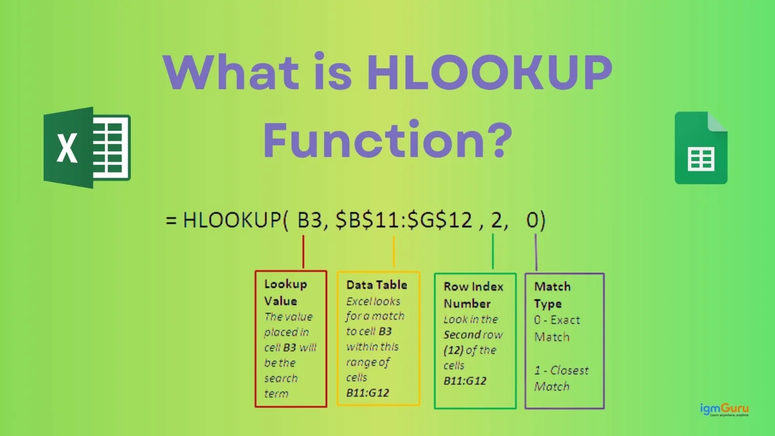
Now that you understand what HLookup does, let’s look at how you actually write it in Excel. Don’t worry, it looks technical at first, but it is very simple once you break it down. Here is the syntax:
|
Let’s understand each part one by one, in a very practical way.
1. Lookup_value: This is the value you want to search for in the first row. It can be a number, text, or even a cell reference. For example, if you are looking for a “Laptop”, this is your lookup value.
2. Table_array: This is the entire range of your data. It includes the top row (where Excel will search) and the rows below (from where it will return the result). Think of it as selecting your full table, not just one row.
3. Row_index_num: This tells Excel which row to return the value from. For example:
So if your prices are in the second row, you will use 2.
4. [range_lookup]: This part is optional, but very important.
Now let’s actually use HLookup in Excel. This is the part where things start to make real sense. Once you do it once, you will see how easy it actually is.
Imagine you have a table where the first row has product names, and the rows below have details like price, quantity, or sales. Now you want to find one specific value quickly. Here’s how you can do it step by step.
Click on the cell where you want Excel to show the answer. This is where your HLookup result will appear.
Type =HLookup( As soon as you type this, Excel will guide you with the arguments.
This is what you are searching for. You can either type it directly (like "Laptop") or select a cell that contains it.
Now select the entire table that contains your data. Make sure you include the first row (where Excel will search) and the rows below.
Tip: You can press F4 after selecting the range to lock it, so it does not change when you drag the formula.
Now tell Excel which row to return the value from. For example, if the value you need is in the second row, type 2.
Type FALSE if you want an exact match. This is what you should use in most cases to avoid wrong results.
Type ) and press Enter. You will instantly get your result. So in simple words, you are telling Excel: “Find this value in the top row, and give me the value from this row.”
Once you practice this a couple of times, it becomes very natural. You will not even need to think about the steps anymore.
Goal: Find the price of the camera
|
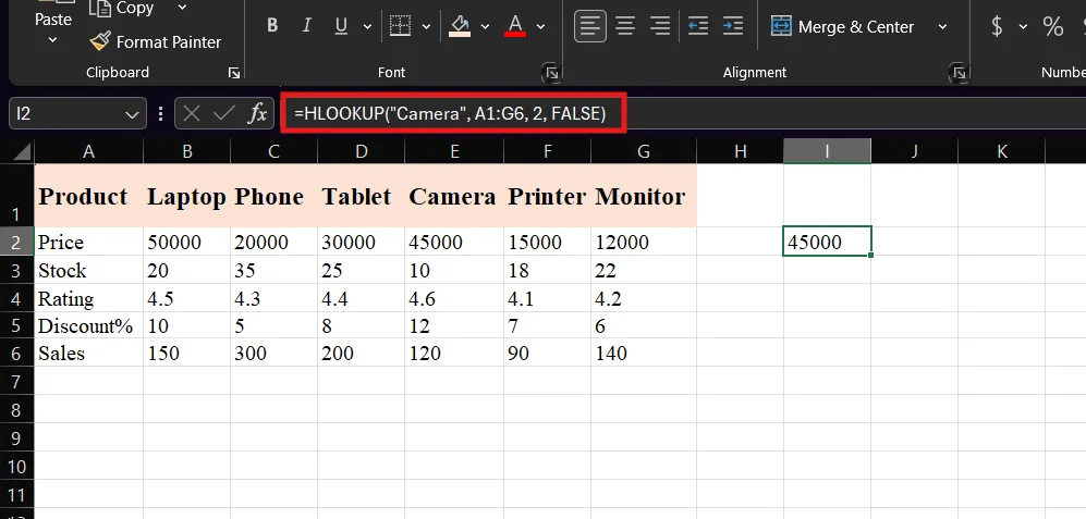
Explanation: Excel searches for "Camera" in the first row of the table. Once it finds it, it moves down to the specified row (Price row). It then returns the corresponding value, which is 45000.
Goal: Find the profit in April
|
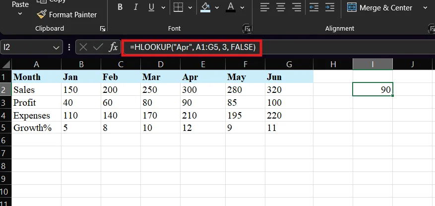
Explanation: Excel searches for "Apr" in the first row. Once it finds it, it moves to the 3rd row (Profit row). It then returns the value, which is 90.
Goal: Find the total marks of Neha
|
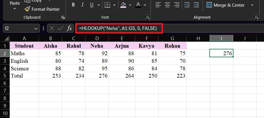
Explanation: Excel looks for "Neha" in the first row. After finding it, it moves to the 5th row (Total row). It then returns the value, which is 276.
Now that you know how to use HLookup, let’s talk about why you would actually use it. Because honestly, no one uses a function just for the sake of it. It should make your work easier, faster, or cleaner. And HLookup does exactly that in the right situations.
1. Works perfectly with horizontal data: If your data is arranged across rows instead of columns, HLookup feels natural. You do not have to rearrange your entire dataset just to make a formula work. It saves time and effort.
2. Simple and easy to understand: The logic behind HLookup is very straightforward. Find a value in the top row, return something from below. Once you understand this flow, it becomes very easy to use even for beginners.
3. Saves time on manual searching: Instead of scrolling through rows and checking values manually, HLookup does it instantly. This is especially helpful when you are working with large datasets.
4. Reduces human error: Manual work always comes with the risk of mistakes. HLookup helps you avoid that by automating the lookup process. Once the formula is correct, your results stay consistent.
5. Can be combined with other formulas: You can use HLookup along with functions like IF, ISNA, or IFERROR. This makes your formulas smarter and more dynamic, especially when handling missing or incorrect data.
6. Useful in reports and dashboards: If you are creating reports where data is structured horizontally, HLookup can quickly pull the required values and make your sheet look clean and professional.
Now let’s be real for a second. HLookup is useful, but it is not perfect. If you understand its limitations early, you will avoid a lot of frustration later.
1. Works only horizontally: HLookup can only search across the first row. If your data is arranged in columns, it simply will not work. In that case, you will have to switch to VLookup or XLookup.
2. Lookup value must be in the first row: This is a big limitation. HLookup only searches the top row of your table. If your lookup value is somewhere else, HLookup cannot find it unless you rearrange your data.
3. Not flexible when structure changes: If you insert or delete rows in your table, your row index number can break. For example, if you were using row 2 and your data shifts, your formula might start returning the wrong result without you noticing.
4. Approximate match can give wrong results: If you use TRUE instead of FALSE, Excel may return the closest match instead of the exact one. This can lead to incorrect answers, especially if your data is not sorted properly.
5. Cannot look to the “left” or above: HLookup only moves downward from the first row. It cannot go above or work in reverse, which makes it less flexible compared to modern functions.
6. Limited compared to XLookup: Newer functions like XLookup are much more powerful. They allow flexible lookup in any direction, do not depend on position, and are easier to manage in complex datasets.
When you start using HLookup, it works great until it suddenly doesn’t. You enter the formula, press Enter, and Excel throws an error. It can feel confusing at first, but most of these errors are very common and easy to fix once you understand them. Let’s go through the ones you will see most often.
This is the most common error. It usually means Excel could not find your lookup value in the first row.
This happens when your row index number is incorrect.
This error appears when Excel does not understand one of your inputs.
Sometimes the formula runs, but the answer is wrong. This is even more dangerous because you might not notice it.
This happens when Excel does not recognize the function.
At some point, almost everyone gets confused between HLookup, VLookup, and XLookup. They all help you find data, but they work in slightly different ways. And honestly, choosing the right one can save you a lot of time and effort. Let’s first understand the basic idea in a simple way:
Now let’s break this down clearly so you can actually decide which one to use.
| Feature | HLookup | VLookup | XLookup |
|---|---|---|---|
| Search Direction | Horizontal (Top Row) | Vertical (First Column) | Both (Any Direction) |
| Lookup Position | Must be in the first row | Must be in the first column | Can be anywhere |
| Flexibility | Low | Medium | High |
| Ease of Use | Simple | Simple | Very Easy |
| Exact Match Default | No (need FALSE) | No (need FALSE) | Yes (default exact match) |
| Can Look Left/Up? | No | No | Yes |
| Breaks When Data Changes? | Yes | Yes | No |
| Requires Column/Row Index | Yes | Yes | No |
| Works in Older Excel Versions | Yes | Yes | Only in newer Excel |
| Error Handling | Manual (IFERROR needed) | Manual | Built-in options |
Now the real question is not just how HLookup works, but when you should actually use it. Because honestly, using the right function at the right time makes all the difference.
HLookup is not something you will use everywhere. But in the right situation, it becomes very helpful and saves you a lot of effort. Let’s understand where it actually makes sense to use it.
1. When your data is arranged horizontally: If your data is spread across rows instead of columns, HLookup is the right choice. For example, when your headings are in the first row and values are below them.
2. When your lookup value is in the first row: HLookup only searches the top row. So if the value you want to find is placed there, this function will work perfectly.
3. When you need a quick and simple solution: If your dataset is small and simple, HLookup is easy to apply. You do not need complex formulas or extra setup.
4. When you are working on older Excel versions: If you are using an older version of Excel where XLookup is not available, HLookup is still a reliable option.
5. When your data structure is fixed: If your table layout is not going to change, HLookup works well. But if your data keeps changing, it may not be the best choice.
6. When you are comfortable with basic Excel functions: If you already understand simple formulas, HLookup is easy to learn and use without much effort.
HLookup is one of those Excel functions that feels simple once you truly get it. It helps you search data across rows and pull the exact value you need without wasting time. It may not be as flexible as newer functions, but it still works really well in the right situations. If your data is arranged horizontally and your lookup value is in the top row, HLookup can do the job quickly and cleanly. At the same time, it is important to understand its limits so you do not rely on it where it does not fit. You just need to learn it well, practice a little, and you will know exactly when to use it.
HLookup is used to search for a value in the first row of a table and return a related value from a row below. It is helpful when your data is arranged horizontally.
HLookup searches across rows, while VLookup searches down columns. The choice depends on how your data is structured.
It usually happens because the lookup value is not in the first row, there is a spelling mistake, or the match type is incorrect. Always check these first.
If you have access to XLookup, it is usually the better option because it is more flexible and easier to use. But HLookup still works well for simple, horizontal data.