What Is a Confusion Matrix in Machine Learning?

You have trained a machine learning model. It looks great on paper. The accuracy is 95%. You are ready to deploy it. But then it fails in production. It misses the very cases you built it for.

This happens more often than you think. In most cases, a confusion matrix could have caught the problem before deployment.

A confusion matrix is one of the most important tools in machine learning. It tells you not just how often your model is right, but exactly where and how it goes wrong. If you work with classification models, understanding the confusion matrix is non-negotiable.

In this guide, you will learn what a confusion matrix is, how it works, how to read it, and how to use it to build better models. We will also walk through a Python implementation and cover real-world applications.

Let us get started!

Also Read: CatBoost in Machine Learning

What is a Confusion Matrix In Machine Learning?

A confusion matrix is a performance evaluation table for machine learning classification models. It compares a model's predicted categories against the actual, true categories of a dataset. Rather than summarizing performance in a single percentage, it reveals exactly where the model makes mistakes and how it confuses classes.

Example of a Confusion Matrix:

Imagine you have built an email classification model that predicts whether an email is Spam or Not Spam.

You test the model on 100 emails and get the following results:

In this example:

• 40 emails were actually spam and correctly predicted as spam.
• 10 emails were actually spam but incorrectly predicted as not spam.
• 5 emails were actually not spam but incorrectly predicted as spam.
• 45 emails were actually not spam and correctly predicted as not spam.

This confusion matrix not only shows the number of correct predictions but also the specific types of errors the model made. Instead of relying solely on an overall accuracy score, you can see whether the model is more likely to miss spam emails or incorrectly flag legitimate emails as spam.

Why Is a Confusion Matrix Important in Machine Learning?

A confusion matrix is important because it provides a detailed view of how a classification model performs. Unlike accuracy, which only shows the percentage of correct predictions, a confusion matrix reveals the exact types of errors a model makes. Comparing predicted labels with actual labels, it helps identify:

• Correct predictions made by the model.
• False positives, where the model incorrectly predicts a positive class.
• False negatives, where the model fails to identify a positive class.
• Class-specific performance is especially important when dealing with multiple classes.

A confusion matrix is particularly valuable when working with imbalanced datasets, where one class appears much more frequently than others. In such cases, a model may achieve high accuracy while still performing poorly on the minority class. The confusion matrix exposes these hidden issues.

Additionally, it serves as the foundation for several important evaluation metrics, including:

• Precision
• Recall
• F1-Score
• Specificity

By analyzing these metrics, data scientists can better understand model strengths and weaknesses, improve classification performance, and make more informed decisions about model selection and optimization.

Related Article: LightGBM (Light Gradient Boosting Machine)

Structure of a Confusion Matrix

Before you can read a confusion matrix correctly, you need to understand how it is built. The layout follows a consistent pattern that every data scientist uses across projects and tools.

A standard binary confusion matrix has four cells arranged in a 2x2 grid. Each cell represents a specific combination of predicted and actual outcomes.

Here is the standard layout:

Understanding the Four Components of a Confusion Matrix

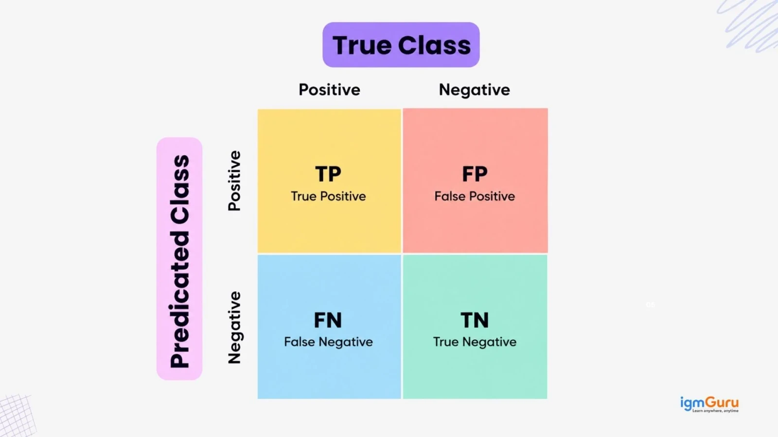
Each cell in the confusion matrix has a specific name and meaning. These four components are the building blocks of every evaluation metric you will use. Understanding them clearly will make the rest of this guide much easier to follow.

1. True Positive (TP)

The model predicted positive, and the actual label is also positive. This is a correct prediction. In the spam example, this means the model correctly identified a spam email as spam.

2. True Negative (TN)

The model predicted negative, and the actual label is also negative. This is also a correct prediction. The model correctly identified a legitimate email as not spam.

3. False Positive (FP)

The model predicted positive, but the actual label is negative. This is a wrong prediction. The model flagged a legitimate email as spam. This is also called a Type I error.

4. False Negative (FN)

The model predicted negative, but the actual label is positive. This is also a wrong prediction. The model missed a real spam email and let it through. This is also called a Type II error.

Understanding these four values is the foundation of everything else. All the metrics you calculate later come directly from these four numbers.

Read Also: How to Install TensorFlow: A Step-by-step Guide For Beginners

How to Interpret a Confusion Matrix?

Having the confusion matrix in front of you is just the first step. Knowing how to read it correctly is what gives you actionable insight. Here is a simple approach you can use every time.

Reading a confusion matrix becomes straightforward once you know what to look for.

• Start with the diagonal

In a correctly structured confusion matrix, the diagonal from top-left to bottom-right contains the correct predictions. Higher numbers on the diagonal mean better model performance.

• Look at the off-diagonal values

These are the errors. Large off-diagonal numbers tell you the model is regularly confusing one class with another.

• Compare row totals

Each row represents an actual class. The row total tells you how many samples belong to that class. If one class has far more samples than another, you are dealing with a class imbalance.

• Ask what each error costs

A false negative in a cancer detection model is far more dangerous than a false positive. A confusion matrix helps you think about the real-world cost of each error type.

Why Accuracy Alone is Not Enough?

Most beginners start with accuracy because it feels simple and intuitive. But accuracy can give you a false sense of confidence, especially when your dataset is not balanced. This section shows you exactly why that happens.

Accuracy is calculated as:

Accuracy measures the total number of correct classifications divided by the total number of cases.

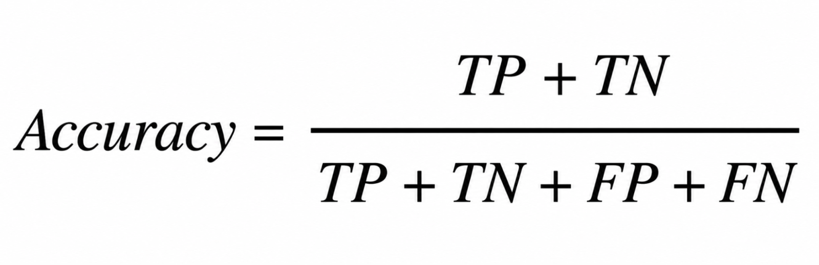
This seems reasonable. But it only tells you the percentage of correct predictions overall.

Consider a fraud detection system. Out of 10,000 transactions, 9,900 are legitimate and 100 are fraudulent. A model that predicts "Not Fraud" for everything achieves 99% accuracy. But it catches zero fraud cases.

This is the accuracy paradox. It is especially common in medical diagnosis, fraud detection, and other high-stakes applications where the minority class is the one that matters most.

The confusion matrix gives you the full picture. It shows you exactly how the model performs on each class separately.

Read Also: What Is PyTorch?

Performance Metrics Derived from a Confusion Matrix

The confusion matrix does not just show you errors. It also unlocks a set of powerful metrics that give you a much deeper view of model performance. Each metric measures something different, and knowing when to use each one is a key skill for any machine learning practitioner.

The four components of a confusion matrix feed directly into these key evaluation metrics.

1. Precision

Precision indicates the proportion of positive predictions made by a model that are accurate.

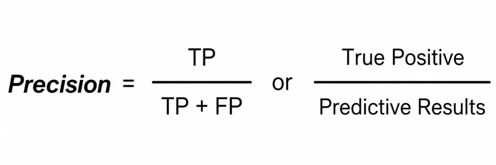
High precision means fewer false positives. This matters when false alarms are costly. For example, you do not want a spam filter that marks important emails as spam too often.

2. Recall (Sensitivity)

Recall measures how many of the actual positive cases the model correctly identified.

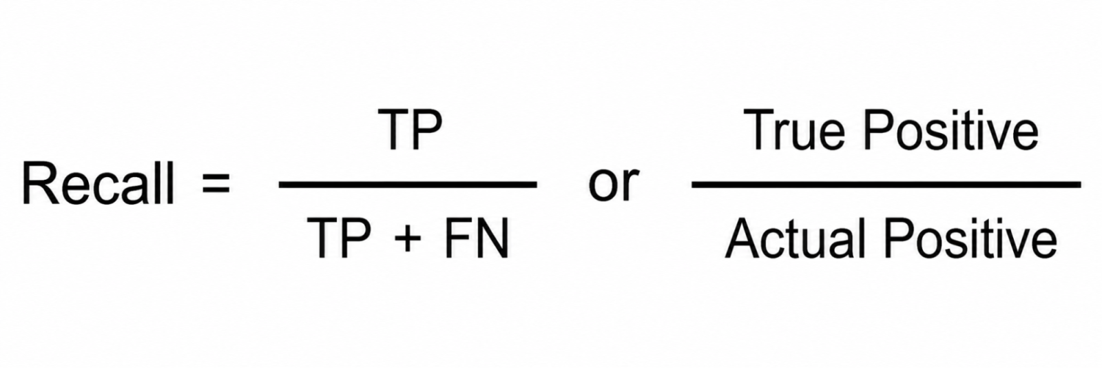
High recall means fewer missed positives. This matters when missing a positive case is dangerous. In cancer screening, missing a true cancer case is far worse than a false alarm.

3. F1-Score

The F1-score is the harmonic mean of precision and recall. It balances both metrics in a single number.

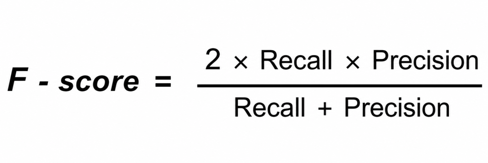
The F1-score is especially useful when you need to balance precision and recall and when the dataset is imbalanced.

Related Article: What Is Machine Learning Operations?

4. Specificity

Specificity measures how well the model identifies negative cases.

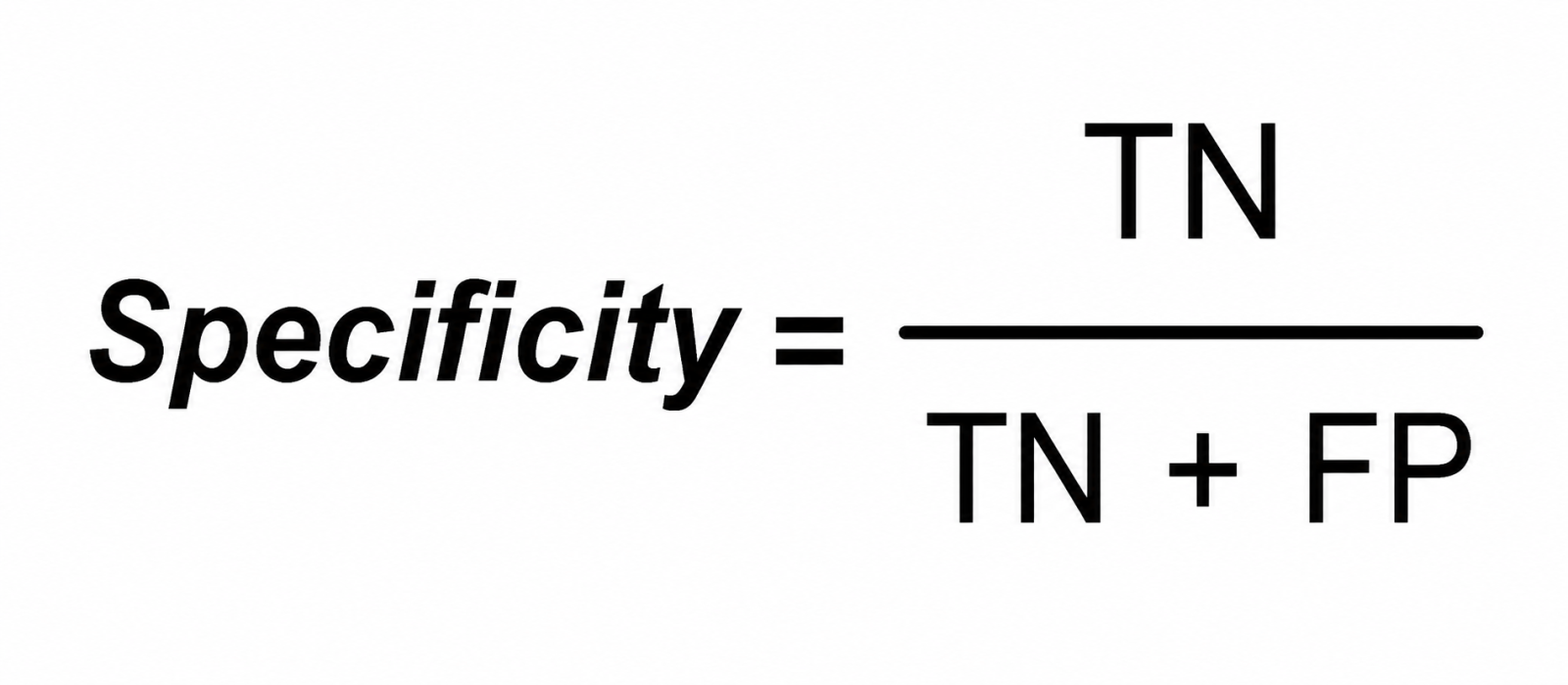
High specificity means fewer false positives. This is important in scenarios where flagging a negative case as positive carries a significant cost.

Which Metric Should You Use?

The right metric depends on your use case:

• Medical diagnosis: Prioritize recall. Missing a disease is worse than a false alarm.
• Spam detection: Balance precision and recall. Use F1-score.
• Fraud detection: Prioritize recall for the fraud class. Use F1-score on the minority class.
• General classification: Use accuracy only when classes are balanced.

Also Read: What is MLOps (Machine Learning Operations)?

Confusion Matrix for Multiclass Classification

Binary classification is just one use case. Many real-world problems involve three or more classes, and the confusion matrix handles them just as well. The structure scales up naturally, though reading it does require a bit more attention.

So far, we have focused on binary classification with two classes. But confusion matrices also work for multiclass problems.

In a multiclass confusion matrix, the rows represent actual classes and the columns represent predicted classes. The size of the matrix grows with the number of classes. For a 3-class problem, you get a 3×3 matrix. For a 10-class problem, you get a 10×10 matrix.

Multiclass Example

Suppose you are building a model to classify animals into three categories: Cat, Dog, and Bird. You test on 30 samples and get this result:

The diagonal shows correct predictions. Off-diagonal values show confusion between classes. Here, the model sometimes confuses cats with dogs and dogs with birds, but never confuses cats with birds.

For multiclass problems, you calculate precision, recall, and F1-score for each class separately. Then you average them using:

• Macro average: Treats all classes equally, regardless of size.
• Weighted average: Accounts for the number of samples in each class. Better for imbalanced datasets.

How to Create a Confusion Matrix in Python?

Theory is important, but seeing it in code makes everything click. Python's scikit-learn library makes it very easy to generate and visualize a confusion matrix in just a few lines. Follow these steps and you will have a working implementation in minutes.

Python makes it easy to create a confusion matrix using scikit-learn. Here is a step-by-step example.

Step 1: Install Required Libraries

pip install scikit-learn matplotlib seaborn

Step 2: Import Libraries

import numpy as np
import matplotlib.pyplot as plt
import seaborn as sns
from sklearn.metrics import confusion_matrix, classification_report
from sklearn.model_selection import train_test_split
from sklearn.linear_model import LogisticRegression
from sklearn.datasets import load_breast_cancer

Step 3: Load Data and Train a Model

# Load dataset
data = load_breast_cancer()
X, y = data.data, data.target

# Split into train and test sets
X_train, X_test, y_train, y_test = train_test_split(
    X, y, test_size=0.2, random_state=42
)

# Train a logistic regression model
model = LogisticRegression(max_iter=10000)
model.fit(X_train, y_train)

# Make predictions
y_pred = model.predict(X_test)

Step 4: Generate the Confusion Matrix

# Create confusion matrix
cm = confusion_matrix(y_test, y_pred)

print("Confusion Matrix:")
print(cm)

Step 5: Visualize the Confusion Matrix

# Plot with seaborn heatmap
plt.figure(figsize=(8, 6))

sns.heatmap(
    cm,
    annot=True,
    fmt='d',
    cmap='Blues',
    xticklabels=data.target_names,
    yticklabels=data.target_names
)

plt.title('Confusion Matrix')
plt.xlabel('Predicted Label')
plt.ylabel('Actual Label')
plt.tight_layout()
plt.show()

Step 6: Get a Full Classification Report

print(
    classification_report(
        y_test,
        y_pred,
        target_names=data.target_names
    )
)

This report gives you precision, recall, F1-score, and support for each class in one output. It is the fastest way to evaluate a classification model in Python.

Read Also: Top Machine Learning Algorithms to Know

Confusion Matrix vs Other Evaluation Metrics

The confusion matrix is a powerful tool, but it works best when you understand how it fits alongside other evaluation metrics. Each metric has a purpose, and knowing which one to use in a given situation will make you a stronger practitioner.

The confusion matrix is not the only evaluation tool. Here is how it compares to others.

The confusion matrix sits at the top of this list because most other metrics are derived from it. You should always start with the confusion matrix before moving to other metrics.

Real-World Applications of Confusion Matrices

Understanding a concept in theory is one thing. Seeing where it gets used in the real world makes it stick. Confusion matrices are not just a classroom tool. They drive decisions in some of the most critical machine learning systems in use today.

Confusion matrices are used across industries wherever classification models exist.

1. Medical Diagnosis

In disease detection, a false negative can be life-threatening. Missing a cancer diagnosis is far worse than a false alarm. Doctors and data scientists use confusion matrices to evaluate recall and minimize false negatives.

2. Email Spam Detection

Spam filters need to balance two risks. Missing spam is annoying. Blocking legitimate email is worse. The confusion matrix helps tune the model to find the right balance.

3. Fraud Detection

Banks and payment companies use confusion matrices to evaluate fraud detection models. The fraud class is a tiny minority, so accuracy is meaningless. The confusion matrix reveals how well the model catches actual fraud without blocking legitimate transactions.

4. Self-Driving Vehicles

Object recognition models in autonomous vehicles must correctly classify pedestrians, vehicles, and road signs. A confusion between a pedestrian and a road sign could be fatal. Confusion matrices help engineers identify and fix these classification errors.

5. Sentiment Analysis

Customer service teams use sentiment classifiers to tag reviews and tickets as positive, negative, or neutral. Confusion matrices help identify which sentiments the model handles well and which it consistently misclassifies.

Related Article: What is Natural Language Processing (NLP)?

Advantages of Using a Confusion Matrix

There are many ways to evaluate a machine learning model. So why does the confusion matrix stand out? Because it gives you information that no other single tool provides. Here are the key advantages that make it a staple of every model evaluation workflow.

A confusion matrix offers several advantages over other evaluation approaches.

1. It reveals error types: You can see not just how many errors the model makes, but what kind of errors and where they occur.
2. Works for any number of classes: Whether you have 2 classes or 20, the confusion matrix scales with your problem.
3. It enables targeted improvement: When you see which classes the model confuses most, you can collect more data for those specific classes or adjust your features.
4. It handles imbalanced data honestly: Unlike accuracy, the confusion matrix does not hide poor performance on minority classes.
5. It is the source of all key metrics: Precision, recall, F1-score, and specificity all come from the confusion matrix. It is the root of your evaluation pipeline.

Limitations of a Confusion Matrix

The confusion matrix is a great tool, but it is not a complete solution on its own. Like any evaluation method, it has blind spots. Knowing these limitations will help you use it more responsibly and pair it with the right complementary tools.

No tool is perfect. The confusion matrix has a few limitations you should know about.

1. It does not capture prediction confidence: The confusion matrix treats a prediction of 51% and 99% confidence equally. It only cares about the final predicted class, not how sure the model was.
2. It becomes harder to read with many classes: A 20×20 confusion matrix is difficult to interpret visually. You need to rely on aggregated metrics like macro-averaged F1-score instead.
3. It does not account for cost differences: Not all errors are equal. A confusion matrix treats every false positive the same way, regardless of the real-world consequence. You need to add cost-sensitive analysis separately.
4. It requires threshold decisions for probabilistic models: For models that output probabilities, you need to set a decision threshold before creating the confusion matrix. Different thresholds produce different matrices.

Also Read: What is Hyperparameter Tuning?

Common Mistakes to Avoid When Using a Confusion Matrix

Knowing what a confusion matrix is and knowing how to use it correctly are two different things. Several common errors can lead you to wrong conclusions. Being aware of them upfront will save you a lot of troubleshooting later.

Even experienced practitioners make these mistakes. Here is what to watch out for.

1. Relying only on the diagonal: Looking at just the correct predictions misses the entire point. Always analyze the off-diagonal values carefully.
2. Ignoring class imbalance: If your dataset is heavily imbalanced, the confusion matrix numbers can look fine while the model is still failing on the minority class. Always check class-specific recall.
3. Using accuracy as your only metric: Accuracy is derived from the confusion matrix but does not tell the full story. Use it alongside precision, recall, and F1-score.
4. Not normalizing the matrix: When dealing with classes that have significantly different sample sizes, normalize the confusion matrix by row. This approach converts raw counts into percentages, providing a clearer view of how well the model performs across each class regardless of class imbalance.
5. Skipping visualization: Raw numbers are harder to interpret than a heatmap. Always visualize your confusion matrix, especially for multi-class problems.
6. Forgetting to set a consistent threshold: If you compare two models using different probability thresholds, the comparison is not valid. Set the same threshold for both.

Best Practices for Using a Confusion Matrix

Avoiding mistakes is a good start. But using the confusion matrix well means going a step further and building good habits around how you apply it. These best practices will help you get reliable, repeatable results every time.

Follow these practices to get the most value from your confusion matrix.

1. Always visualize the data whenever possible: A heatmap that incorporates color intensity and annotations can make hidden patterns, correlations, and trends immediately visible, allowing for faster and more effective data analysis.
2. Normalize when classes are imbalanced: Divide each row by its total to get percentage-based performance per class.
3. Calculate all derived metrics: Do not stop at the matrix itself. Compute precision, recall, and F1-score for every class.
4. Interpret errors in context: Ask what each type of error means in your specific domain. A false negative in fraud detection is not the same as a false negative in product recommendation.
5. Track the confusion matrix over time: As your model or data changes, the confusion matrix will shift. Monitor it regularly to catch performance degradation early.
6. Use it during cross-validation: Do not evaluate only on a single test set. Average confusion matrices across multiple folds for a more reliable assessment.
7. Compare confusion matrices between models: When you are choosing between two classifiers, side-by-side confusion matrices often reveal differences that aggregate metrics miss.

Related Article: Deep Learning vs Machine Learning: Beginner's Guide

Wrapping Up

The confusion matrix is one of the most powerful and practical tools in machine learning evaluation. It gives you a clear, honest breakdown of how your classification model performs on every class, not just overall.

You now know what a confusion matrix is, how to read it, and how to build one in Python. You also know the four core components, the derived metrics that come from them, and how to apply all of this to real-world problems.

Next time you evaluate a classification model, start with the confusion matrix. Use it to guide your decisions about model selection, threshold tuning, and performance improvement.

Good models are not just accurate. They fail in the right places for the right reasons. The confusion matrix helps you confirm that.

FAQs

1. Explain the difference between precision and recall.

Precision measures how many of the model's positive predictions are actually correct. Recall measures how many of the actual positive cases the model successfully identified. Precision focuses on false positives. Recall focuses on false negatives.

2. When should I use F1-score instead of accuracy?

Use the F1-score when your dataset is imbalanced, meaning one class appears far more often than the other. Accuracy can be misleading in these type of situations. The F1-score balances precision and recall and gives a fairer picture of model performance.

3. What is a normalized confusion matrix?

A normalized confusion matrix divides each cell by the total number of actual samples in that class. This converts raw counts into percentages, making it easier to compare performance across classes with different sample sizes.

4. What does a good confusion matrix look like?

A good confusion matrix has high values along the main diagonal and low values everywhere else. This means the model makes correct predictions for most samples in every class with few misclassifications.