Pandas Cheat Sheet

Struggling to manage messy or unorganized data? Pandas can fix that. No, not the animal, but the powerful Python library trusted for data manipulation, cleaning, transformation and analysis. It lets you handle large datasets in seconds with a few lines of code, making it essential in modern data work.

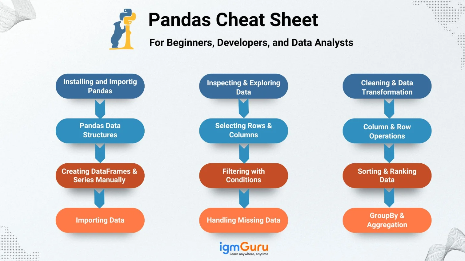
This Pandas cheat sheet will guide you step-by-step with clear explanations and practical examples based on real use cases. No theory overload, no confusing jargon, just hands-on Pandas you can apply immediately to level up your data skills. It will be the best toolkit for:

• Beginners and learners entering data analysis
• Python users who want to work with real datasets
• Students preparing for assignments, projects, or internships
• Data analysts, aspiring data scientists, and ML beginners
• Professionals looking for a quick refresher

What is Pandas?

Pandas is a Python library built for fast and flexible data management. It makes it easier to load, view, clean, filter, transform, reshape, merge, and analyze structured datasets like CSV, Excel, SQL exports, and JSON files. It behaves like a spreadsheet but runs with Python’s speed, logic, and automation power.

It helps discover patterns, summarize metrics, process large files, and prepare data for machine learning. Looking complicated? Do not worry, it is an easy-to-understand library for everyone, from beginners to experienced professionals. That is why it is used by data analysts, data scientists, researchers, developers, and many others.

It also allows quick transformations without manual effort and reduces time spent in raw data handling, so you can focus on analysis instead of struggling with formats, errors, and repetitive cleaning tasks.

Example

import pandas as pd

# Load a dataset (example file)
df = pd.read_csv("students.csv")

print(df.head())   # preview first 5 rows

Related Article: Python Cheat Sheet

Installing and Importing Pandas

Pandas is not a default Python library. You have to add it using the pip or conda method. The common import method is import pandas as pd so functions can be typed quickly. After installation, Pandas integrates smoothly with NumPy, Matplotlib, scikit-learn, and Jupyter notebooks.

You can check the version, confirm installation success, and begin using DataFrames instantly. The best part is that Pandas installation rarely fails and setup usually takes only a few seconds. Just run the following commands and start working with your data efficiently.

Example

pip install pandas          # using pip
# or
conda install pandas        # using conda

import pandas as pd         # import after installation
print(pd.__version__)       # check installed version

Pandas Data Structures (Series & DataFrame)

Pandas relies mainly on two data structures, Series and DataFrame. A Series is a one-dimensional array with labels, ideal for column-like data. A DataFrame is a table made of multiple Series stacked as columns, closely resembling Excel sheets or SQL tables in daily analytics workflows.

Nearly all Pandas functions return or modify Series or DataFrames, so knowing both is fundamental. DataFrames allow indexing, slicing, grouping, merging, sorting, and aggregating with minimal code. Series underlie DataFrames, and mastering them gives deeper control over transformations and custom logic.

Example

import pandas as pd

# Series
marks = pd.Series([88,92,75,90], name="Score")
print(marks)

# DataFrame
df = pd.DataFrame({
    "Name":["Amit","Rekha","Iram","Karan"],
    "Score":[88,92,75,90],
    "Grade":["A","A","B","A"]
})

print(df)

Creating DataFrames & Series Manually

DataFrames can be generated from dictionaries, lists, arrays, or nested structures. Creating them manually is useful for practice, prototyping, and testing transformations before applying them to large files. Pandas automatically assigns an index, but you may set your own custom row labels when needed.

Understanding manual DataFrame creation speeds up debugging and allows flexible experimentation. You can quickly build small in-memory datasets, try out group operations, perform joins, or test cleaning strategies without waiting for big files to load from disk or databases.

df.shape

df = pd.read_csv("file.csv")

df.dtypes

df.head()

df.tail()

df.describe()

Example

data = {
    "Product":["Shoes","Bags","Watch","Perfume"],
    "Price":[1500,2500,3400,2200],
    "Stock":[42,18,12,15]
}

inventory = pd.DataFrame(data)

print("Complete Inventory List:")
print(inventory)

df = pd.DataFrame(data)

s = pd.Series(data)

idx = pd.Index(["A","B","C"])

Importing Data (CSV / Excel / JSON / SQL)

Now let us come to the main deal, data extraction. It is the first thing a data analyst must do, because real work begins with importing files. Pandas reads CSV, Excel, JSON, SQL database tables and more, helping you connect to most common structured data formats in one place.

The most common method is read_csv, which supports encoding, missing value interpretation, custom delimiters, selective column loading, and header control. read_excel allows sheet selection and flexible options. These functions make reading raw datasets much simpler than manual parsing or ad-hoc scripts.

Example

# CSV import with NA handling
df = pd.read_csv("sales.csv", sep=";", na_values=["NA","--"])

# Read specific Excel sheet
orders = pd.read_excel("orders.xlsx", sheet_name="2025_Sales")

print(df.head())
print(orders.head())

import pandas as pd

df = pd.read_csv("file.csv")

df = pd.read_table("file.txt")

df = pd.read_excel("file.xlsx")

df = pd.read_sql("SELECT * FROM table", conn)

df = pd.read_json("file.json")

df = pd.read_html("https://example.com")

df = pd.read_clipboard()

Inspecting & Exploring Data

The next step is to explore your data carefully before modifying it. It might feel boring sometimes, but it is essential to ensure that the dataset is valid, complete, and well-structured. A quick inspection helps you catch missing values, strange distributions, and incorrect formats early.

Pandas offers summary statistics, data type information, row counts, missing value checks, and basic distribution understanding. info() shows column types and memory usage, while describe() summarizes numerical features with mean, standard deviation, minimum, maximum, and percentile values.

Example

df = pd.read_csv("employees.csv")

print(df.head(10))     # sample data preview
print(df.info())       # datatype + memory profile
print(df.describe())   # summary stats

Selecting Rows & Columns

As you move further in data analysis, selection operations become more critical and mistakes can cause serious issues. Column selection and row extraction are core skills. Use bracket syntax to extract columns. .loc selects rows by labels, while .iloc selects rows using integer positions.

You can also use combined indexing to retrieve multi-column slices, specific subsets, conditional rows, and structured views for analysis. Proper selection powers filtering, grouping, transformations, and reporting with precision, making your workflows both readable and efficient.

Example

# Select columns
print(df["Salary"])
print(df[["Name","Salary","Department"]])

# Row selection by positions
print(df.iloc[5:12])

# Selection using label condition
print(df.loc[df["Department"]=="IT"])

Filtering with Conditions

What if your data is impure or contains irrelevant records? Conditional filtering helps you keep only the rows that matter. It returns records matching specific criteria using comparison operators, logical operators, membership checks, or string-based filters.

Conditional filtering is the backbone of cleaning, segmentation, risk detection, anomaly spotting, and KPI analysis. When combined with chaining and grouping, filters form powerful pipelines that reveal patterns and focus your attention on the most important segments of the dataset.

Example

# Employees older than 30
age_filter = df[df["Age"]>30]

# Multiple conditions
filtered = df[(df["Department"]=="IT") & (df["Salary"]>70000)]

print(age_filter)
print(filtered)

Handling Missing Data

Incorrect or missing data can silently break your analysis if ignored. Missing values disrupt calculations, averages, and model training. Pandas identifies nulls using isna() or isnull(). You may drop missing records entirely or fill them based on intelligent strategies.

Common fill strategies include mean, median, mode, forward fill, backfill, or constant replacement. Clean handling of missing values ensures correct statistics, fair machine learning models, and consistent behavior across columns, especially when merging multiple noisy data sources.

Example

# Fill age with mean
df["Age"] = df["Age"].fillna(df["Age"].mean())

# Drop rows where Salary missing
df = df.dropna(subset=["Salary"])

print(df.isna().sum())

Cleaning & Data Transformation

Cleaning focuses on adjusting inconsistent values, text casing, typographical issues, abbreviations, and formatting mistakes. Transformation changes the structure, converts data types, encodes labels, applies formulas, replaces strings, or maps categories. Together, these steps shape raw data into a reliable analysis-ready form.

Most data analysis time is spent on cleaning and transformation. Although it may feel repetitive, clean data leads to more accurate insights, better dashboards, and high-quality machine learning features. Careful transformations also improve reproducibility and trust in your final reports.

Example

# Title case names
df["Name"] = df["Name"].str.title()

# Fix department labels
df["Department"] = df["Department"].replace({"HR":"Human Resources","IT":"Technology"})

# Annual salary from monthly
df["AnnualSalary"] = df["Salary"]*12

print(df.head())

Column & Row Operations

Columns in a DataFrame can be added, updated, renamed, or removed as your analysis evolves. Rows can be sliced, appended, sorted, or reindexed. Setting a meaningful index or resetting the default index can improve performance and readability during merges, joins, and advanced filtering.

Column-level work is the spine of Pandas data wrangling. Most calculated metrics, indicators, or feature engineering steps are expressed as new or transformed columns, making it crucial to understand how to manipulate them safely and efficiently.

Example

# Add column
df["Bonus"] = df["AnnualSalary"]*0.10

# Rename column
df = df.rename(columns={"AnnualSalary":"Yearly_Salary"})

# Delete column
df = df.drop(columns=["Bonus"])

print(df)

Sorting & Ranking Data

Sorting brings order and clarity to your data. You can sort by one or multiple columns, control ascending or descending order, and even sort by index when necessary. Sorted data simplifies reporting, charting, and comparing performance across categories or time periods.

Ranking assigns positions based on column values and is useful for leaderboards, grading, percentile scoring, and competition-style evaluations. With ranking, you can quickly find top performers, bottom performers, or relative standing within groups in your dataset.

Example

sorted_df = df.sort_values(by="Salary", ascending=False)

df["ExperienceRank"] = df["Experience"].rank(ascending=False)

print(sorted_df.head())
print(df.head())

GroupBy & Aggregation

groupby() clusters records that share common values and then applies aggregations. It is extremely useful for department analytics, region-wise revenue, product-wise sales, or customer category patterns. With just a few lines of code, you can build powerful summary tables.

Aggregation functions include mean, sum, count, minimum, maximum, standard deviation, and custom functions. Multi-aggregation summary tables enhance reporting clarity and make it easier for stakeholders to understand performance at different levels of granularity.

Example

dept_salary = df.groupby("Department")["Salary"].mean()

summary = df.groupby("Department").agg({
    "Salary":["mean","max","min"],
    "Experience":"sum"
})

print(dept_salary)
print(summary)

Merging, Joining & Concatenation

Real-world projects often rely on multiple datasets that need to be combined. merge() works like SQL joins on columns, join() merges using indexes, and concat() stacks DataFrames vertically or horizontally. Choosing the correct join type is critical to avoid losing important records.

Data combination builds complete analytical models by combining dimensions like customers, products, and transactions. Whether you are enriching a dataset with extra attributes or stitching together time-based chunks, these functions simplify multi-source integration dramatically.

Example

employee_details = pd.DataFrame({"ID":[101,102,103], "Name":["Amit","Sara","Joel"]})
salary_data      = pd.DataFrame({"ID":[101,102,104], "Salary":[70000,85000,60000]})

merged = pd.merge(employee_details, salary_data, on="ID", how="outer")
print(merged)

Reshaping Data — Pivot & Melt

Reshaping data helps you switch between different views of the same information. pivot() reshapes data from long format to wide format, turning unique values into columns. melt() does the reverse, turning columns into rows for flexible processing.

Reshaping is essential for time series, sales analytics, multi-product comparisons, matrix-style reporting, and visual dashboards. By rearranging data, you can match the structure required by visualization tools, models, or custom business rules.

Example

sales = pd.DataFrame({
    "Month":["Jan","Jan","Feb","Feb"],
    "Product":["Shoes","Bags","Shoes","Bags"],
    "Revenue":[34000,22000,38000,27000]
})

pivoted = sales.pivot(index="Month", columns="Product", values="Revenue")
print(pivoted)

Working with Dates & Times

Datetime fields must be converted into Pandas datetime type for accurate slicing, filtering, time grouping, and resampling. Once converted, you can easily extract year, month, day, weekday, and other components using the .dt accessor and its convenient attributes.

Resampling aggregates values over custom frequency blocks like monthly or weekly and is widely used in forecasting, dashboards, and trend reports. With a proper datetime index, operations like rolling averages or period comparisons become much easier to implement.

Example

df["Date"] = pd.to_datetime(df["Date"])

df["Year"] = df["Date"].dt.year
df["Month"] = df["Date"].dt.month

monthly_salary = df.resample("M", on="Date")["Salary"].sum()
print(monthly_salary)

String Operations

String cleanup is crucial because text fields often contain inconsistent formatting, extra spaces, or mixed casing. Pandas .str methods provide tools for trimming, casing, replacing, splitting, extracting substrings, and performing regular expression searches directly on entire columns.

Clean strings are easier to group, filter, and categorize. Proper text preprocessing prepares columns for modeling, deduplication, segmentation, and downstream analytics, especially when you work with city names, product descriptions, or user-entered comments.

Example

df["City"] = df["City"].str.strip().str.lower()
df["CityCode"] = df["City"].str[:3]

print(df.head())

Plotting with Pandas

Pandas uses Matplotlib as its plotting backend, giving you quick visualizations without manually configuring complex chart objects. It is ideal for fast exploratory analysis where you want to understand distributions, trends, and relationships before building full dashboards.

You can generate histograms, boxplots, bar charts, line charts, and scatter plots from DataFrame columns. Visualizations reveal distribution patterns, outliers, category trends, and correlations far faster than reading raw tables of numbers.

Example

df["Salary"].plot(kind="hist", bins=10, title="Salary Distribution")

Exporting Data (CSV / Excel / JSON)

Exporting the final output is essential after cleaning and analysis. Pandas allows exporting with or without index, custom delimiters, chosen encoding, and multiple file formats. These exported files can be used by BI dashboards, automation pipelines, or other applications.

Whether you are saving intermediate results or production-ready reports, exporting ensures your work is reusable. You can also chain analyses together by feeding exported outputs into other scripts, tools, or cloud services.

Example

df.to_excel("final_report.xlsx", index=False)
df.to_csv("cleaned_data.csv", index=False)

df.to_csv("file.csv", index=False)

df.to_excel("file.xlsx", index=False)

df.to_sql("table_name", conn)

df.to_json("file.json")

df.to_html("file.html")

df.to_clipboard()

Performance Optimization

For large datasets, performance optimization becomes very important. Vectorized operations are much faster than Python loops. Converting string-heavy columns to category type reduces memory usage and often speeds up grouping and filtering operations significantly.

Chunk loading lets you process millions of rows without fully loading them into memory. Avoid row-wise apply() when possible and prefer built-in functions like map(), replace(), or arithmetic operations that leverage Pandas and NumPy internals for speed.

Example

df["Department"] = df["Department"].astype("category")

for chunk in pd.read_csv("bigfile.csv", chunksize=50000):
    print(chunk.shape)

Common Errors & Their Fixes

New users often face errors like KeyError, SettingWithCopyWarning, datatype mismatches, index errors, and column-not-found issues. These errors usually come from typos, chained indexing, or incorrect assumptions about the current DataFrame structure.

Checking column names, copying DataFrames explicitly, and ensuring correct join keys avoids most problems. Reading the error trace carefully and inspecting intermediate results will usually clarify the cause and guide you toward the correct fix quickly.

Example

df = df.copy()  # avoids chained assignment warning

if "Bonus" in df.columns:
    print(df["Bonus"])   # safe lookup

Basic Problems for Practice

Learning any programming concept is not a task of a few hours or days. It requires continuous practice and dedication to strengthen your logical abilities and technical skills. Keeping that in mind, here are some simple but effective practice problems to build confidence with Pandas.

Practice Problems

1. Load a CSV file and display the first 10 rows.
2. Check the number of rows, columns, and datatypes in the dataset.
3. Select only two specific columns from the DataFrame.
4. Filter rows where a numeric column exceeds a given value.
5. Replace missing values in one column using mean or median.
6. Add a new column calculated from two existing ones.
7. Rename two columns to more meaningful names.
8. Sort the DataFrame by one column, then by two columns combined.
9. Group data by a category column and compute average values.
10. Merge two DataFrames on a common key and export the result to CSV.

Wrapping Up

Pandas remains one of the most essential tools for data analysis in Python. It gives you the flexibility to clean, structure, explore, visualize, and export data in a fast and controlled way. With this cheat sheet, you now have a strong foundation for working confidently with real-world datasets.

The key to mastering Pandas is consistent practice. Load different files, experiment with filters, reshape tables, and build your own analysis pipeline. Each dataset you handle will sharpen your understanding and expand your skill set, helping you navigate Pandas with speed and intuition.

FAQs

1. Is Pandas suitable for large datasets?

Yes. Pandas can process large datasets efficiently, especially when you optimize with vectorized operations, chunk reading, appropriate datatypes, and by avoiding unnecessary Python loops. For extremely large data, you can combine Pandas with databases or big data tools.

2. Do I need to know NumPy before learning Pandas?

Not necessarily. Pandas is built on top of NumPy, but beginners can learn Pandas directly and still be productive. Over time, understanding NumPy helps with performance optimization, array manipulation, and advanced operations, but it is not a strict prerequisite.

3. What is the best way to learn Pandas effectively?

The best way is to practice on real datasets. Load files, clean missing values, slice rows, group categories, visualize patterns, and export results. Build simple projects like sales analysis, survey processing, or CSV automation scripts to apply concepts in realistic scenarios.

Articles You Can Also Read:

• Pandas Interview Questions And Answers

• Java Cheat Sheet

• Rust Cheat Sheet

• NumPy Cheat Sheet for Beginners and Developers

• Data Structures in Python

Couse Schedule