Subtraction is one of the most fundamental operations you will ever perform in Excel. Whether you are calculating profit margins, tracking budget variances, measuring time differences, or comparing sales data, knowing how to subtract in Excel quickly and correctly is a skill every spreadsheet user needs.
Here is the important thing to know upfront: Excel does not have a built-in SUBTRACT function. Instead, it uses the minus sign (-) operator directly in formulas. This keeps things simple, but the power comes from knowing all the ways you can apply it, across single cells, entire columns, percentages, dates, times, and more.
This guide covers every method, from the most basic formula to advanced scenarios, with practical examples you can use immediately.
The simplest subtraction formula in Excel follows this structure:
= number1 - number2 |
Example: subtracting hard-coded numbers:
= 500 - 150 |
Result: 350
Example: subtracting with multiple values:
= 500 - 100 - 50 - 30 |
Result: 320
Excel follows PEMDAS (Parentheses, Exponents, Multiplication/Division, Addition/Subtraction). When you mix operations, parentheses determine what gets calculated first:
= (500 - 100) / (80 - 20) |
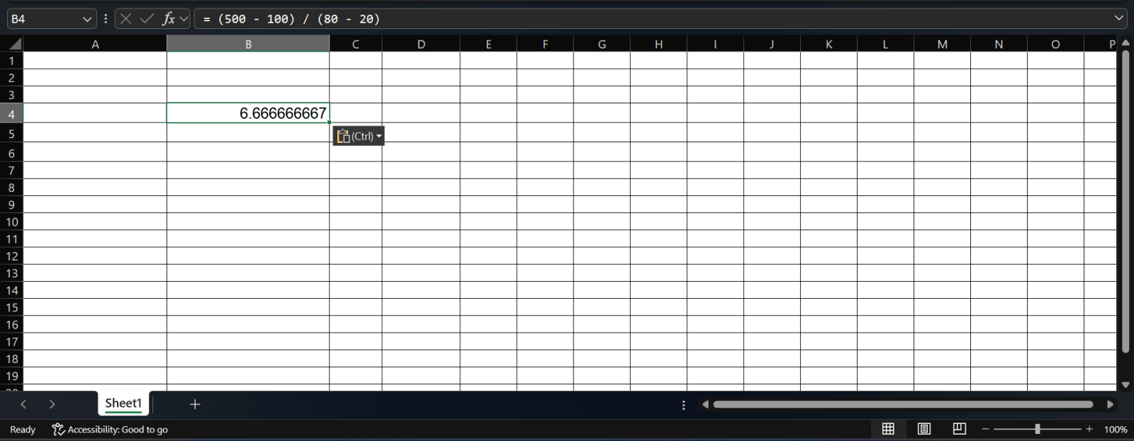
Without parentheses, Excel would divide 100 by 80 first, then handle the subtractions, giving a completely different result. Always use parentheses when combining operations.
Also Read: What is Power Query?
Rather than typing numbers directly into a formula, the smarter approach is to reference the cells that contain those values. This way, if your source data changes, the result updates automatically.
Syntax:
= cell1 - cell2 |
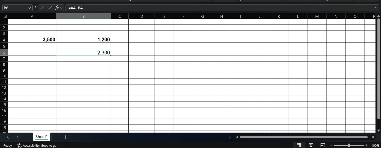
Example: If A4 contains 3,500 and B4 contains 1,200, enter this in C4:
= A4 - B4 |
Result: 2,300
Step-by-step:
Method 1: Chained minus signs:
= B1 - B2 - B3 - B4 - B5 |
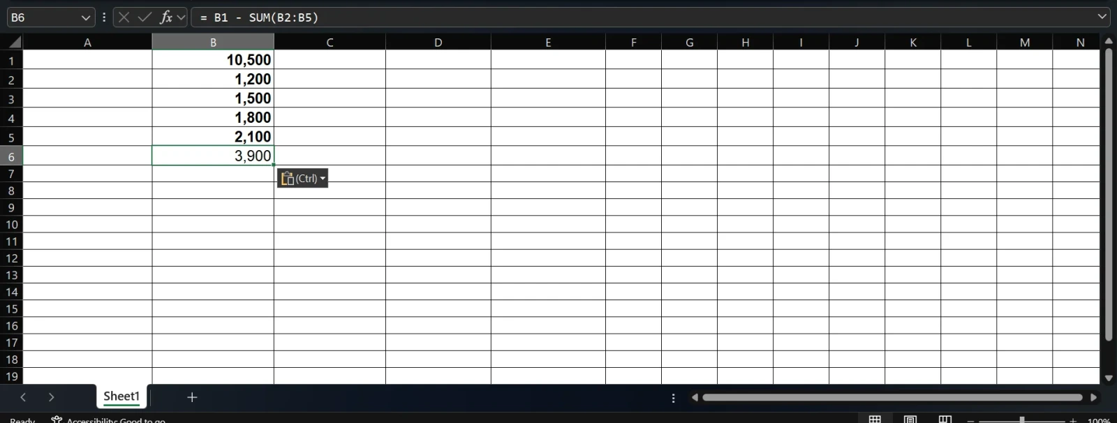
Method 2: Using SUM (cleaner and more scalable):
= B1 - SUM(B2:B5) |
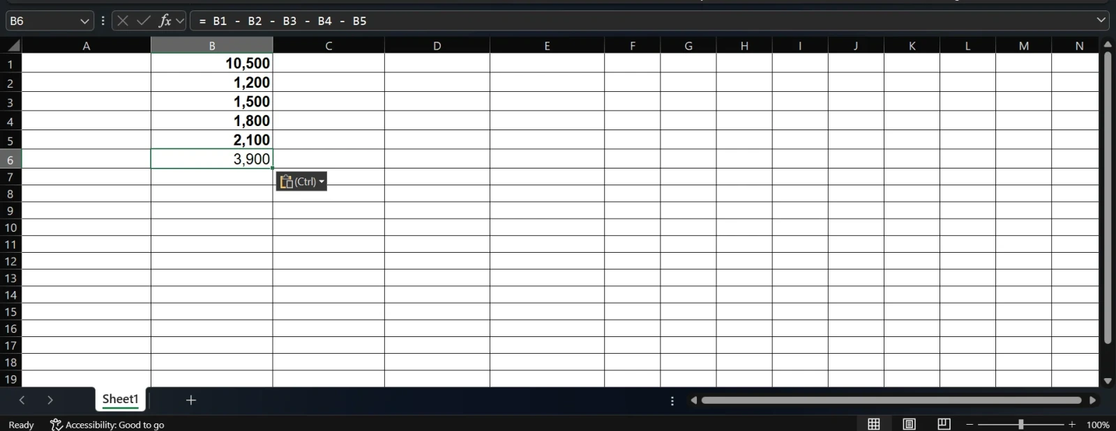
Method 2 is preferred for longer lists as it is easier to read and maintain.
Read Also: How to Create a Dashboard in Excel? A step-by-step Guide
When you have two columns of data and need to subtract each row, you do not need to type a formula for every row. Write one formula and copy it down.
Example:
In D2, enter:
= C2 - B2 |
Then drag the fill handle (small square at the bottom-right of D2) down to D10 (or however far your data goes). Excel automatically adjusts the row references for each row.
Result:
D2 = C2 - B2 |
D3 = C3 - B3 |
D4 = C4 - B4 |
...and so on. |
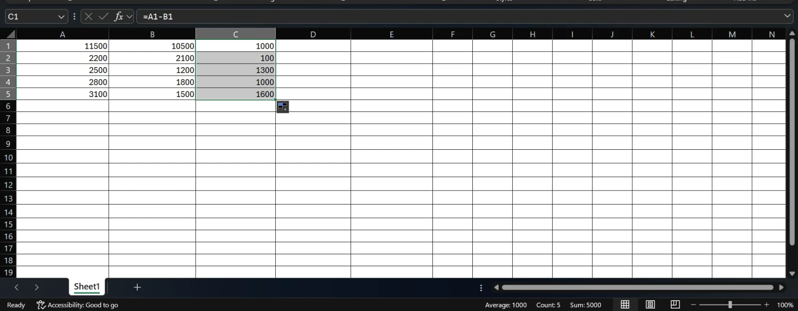
Tip: Double-clicking the fill handle (instead of dragging) automatically fills the formula down to the last row that has data, a big time saver on large datasets.
Related Article: How to Compare Two Columns in Excel?
Sometimes you need to subtract the same number from every value in a column, for example, applying a flat deduction, discount, or tax adjustment across all rows.
Put the deduction amount in cell B2 (e.g., 500). Then in B2:
= A2 - $B$2 |
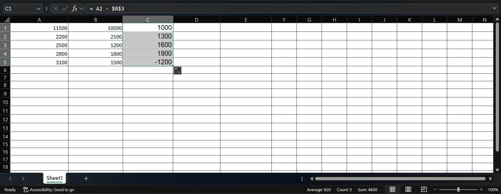
The $ signs lock the reference to E2, so when you copy the formula down, A2 becomes A3, A4, etc., but $E$2 always stays fixed.
= A2 - 500 |
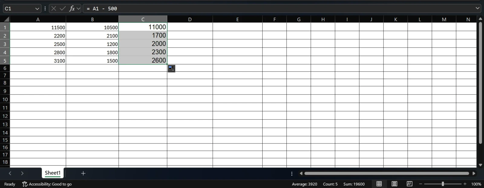
This works, but Method 1 is more flexible. If the deduction amount changes, you update one cell (E2) instead of editing every formula in the column.
= A2 - B2 |
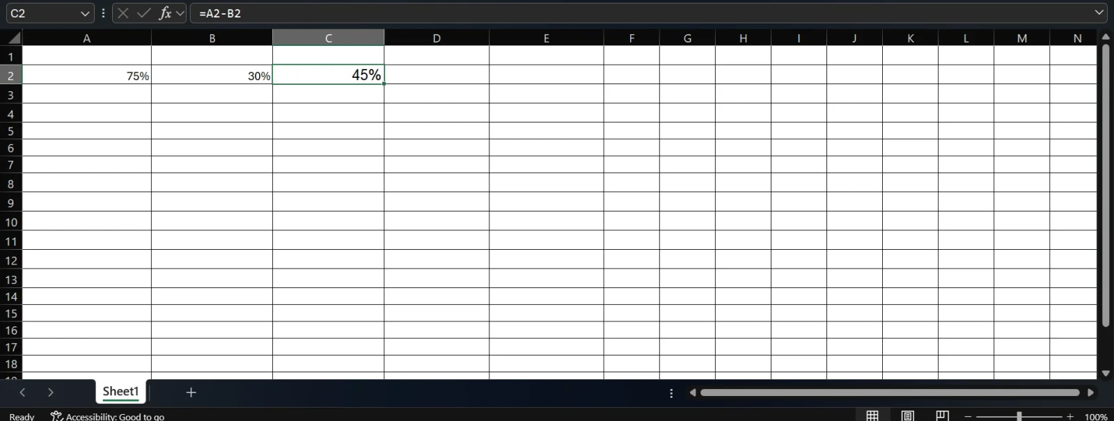
If A2 is 75% and B2 is 30%, the result is 45%.
= A2 * (1 - 20%) |
= A2 * (1 - B2) |
Example: A2 = 8,000 (original price), B2 = 20% (discount).
= 8000 * (1 - 20%) |
Result: 6,400
This formula works by first calculating what remains after the discount (80% of the original), rather than subtracting 20% separately, which is mathematically the same and simpler to read.
Also Read: XLOOKUP() vs. VLOOKUP()
= (B2 - A2) / A2 |
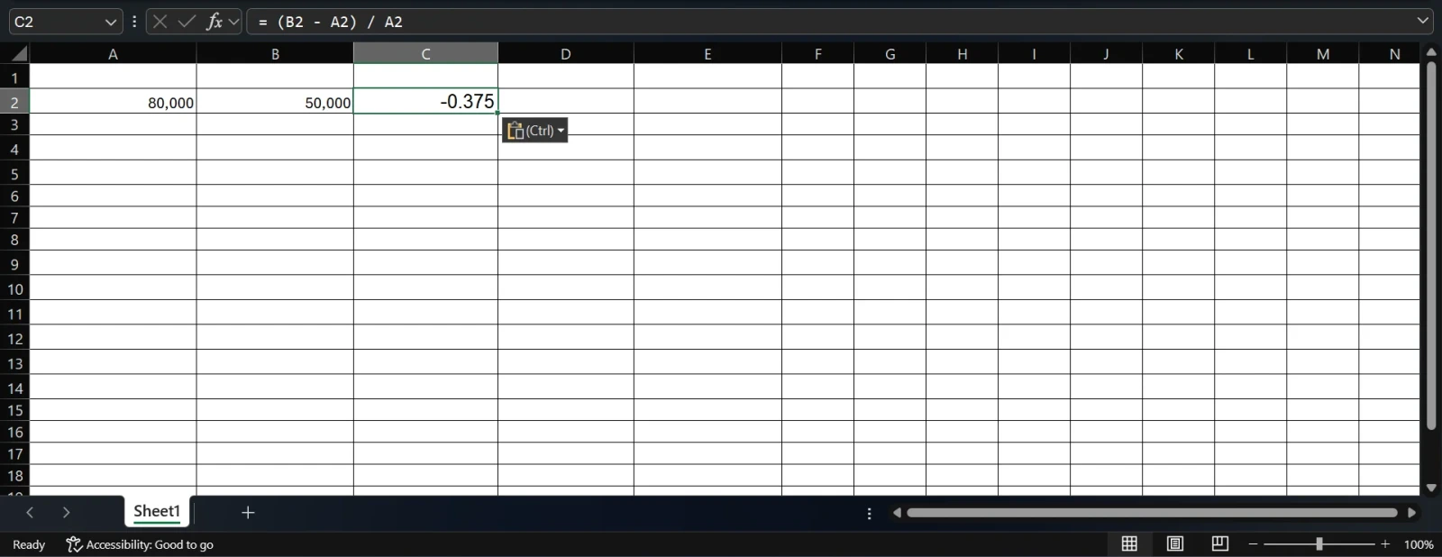
Format the result cell as a percentage to display it correctly.
Excel stores dates as serial numbers (number of days since January 1, 1900), which means subtracting one date from another returns the number of days between them.
= B2 - A2 |
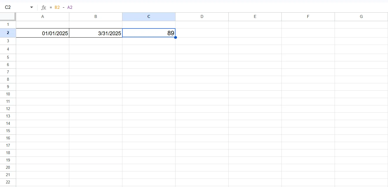
If A2 is 01/01/2025 and B2 is 31/03/2025, the result is 89 (days).
Important: Make sure the result cell is formatted as a Number, not a Date. If it shows a date-like value instead of a number, right-click the cell → Format Cells → select Number.
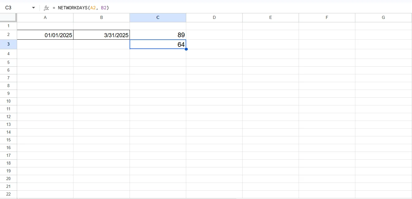
= NETWORKDAYS(A2, B2) |
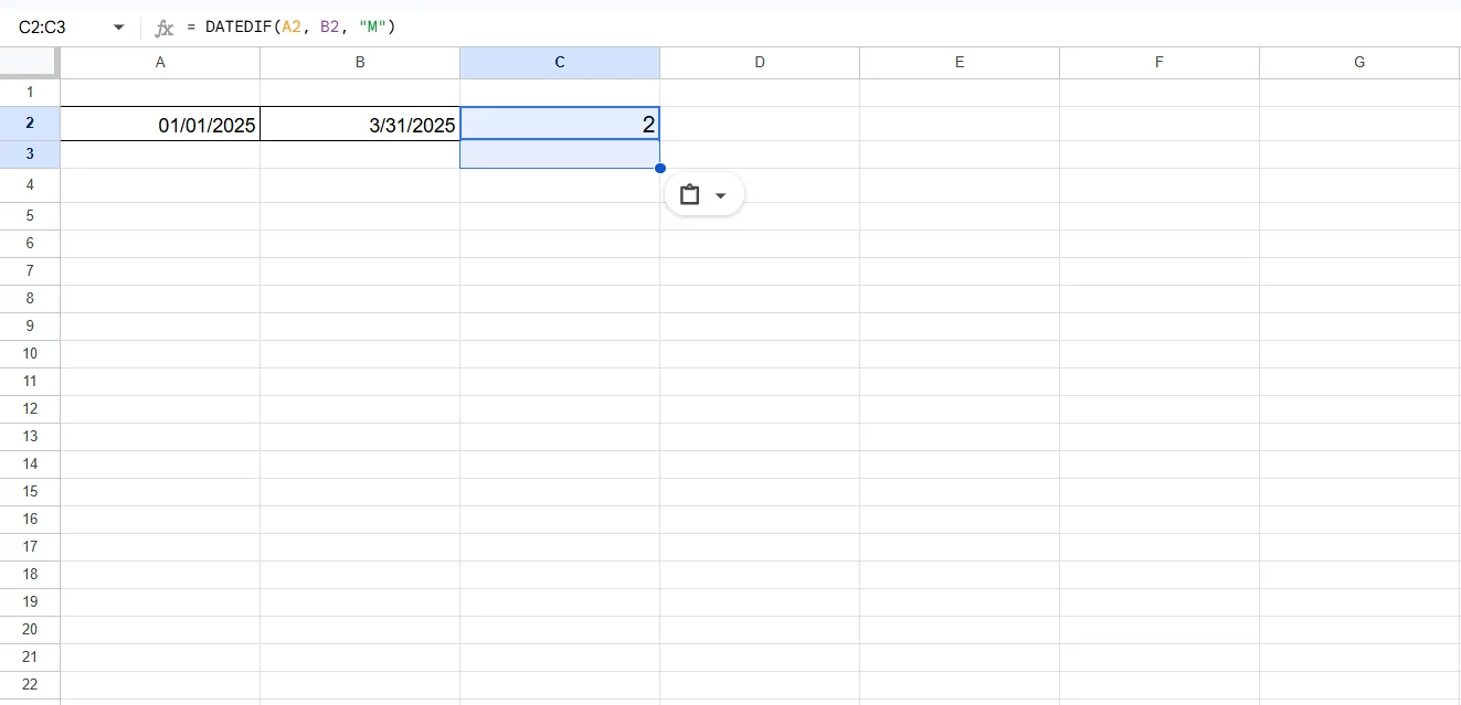
= DATEDIF(A2, B2, "M") |
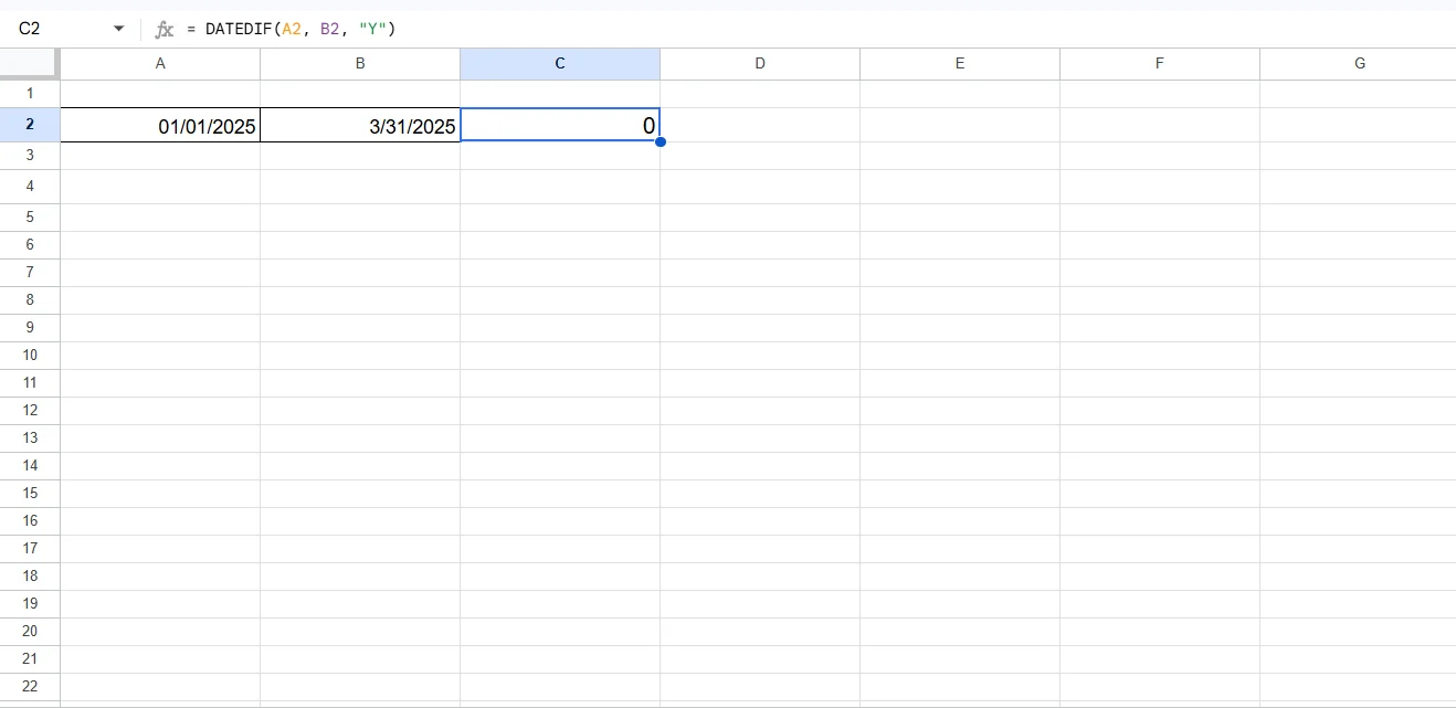
= DATEDIF(A2, B2, "Y") |
Read Also: How to Remove Spaces in Excel?
Just like dates, Excel stores time as decimal fractions of a day (1 hour = 1/24, 1 minute = 1/1440). This means you can subtract times the same way you subtract dates.
= B2 - A2 |
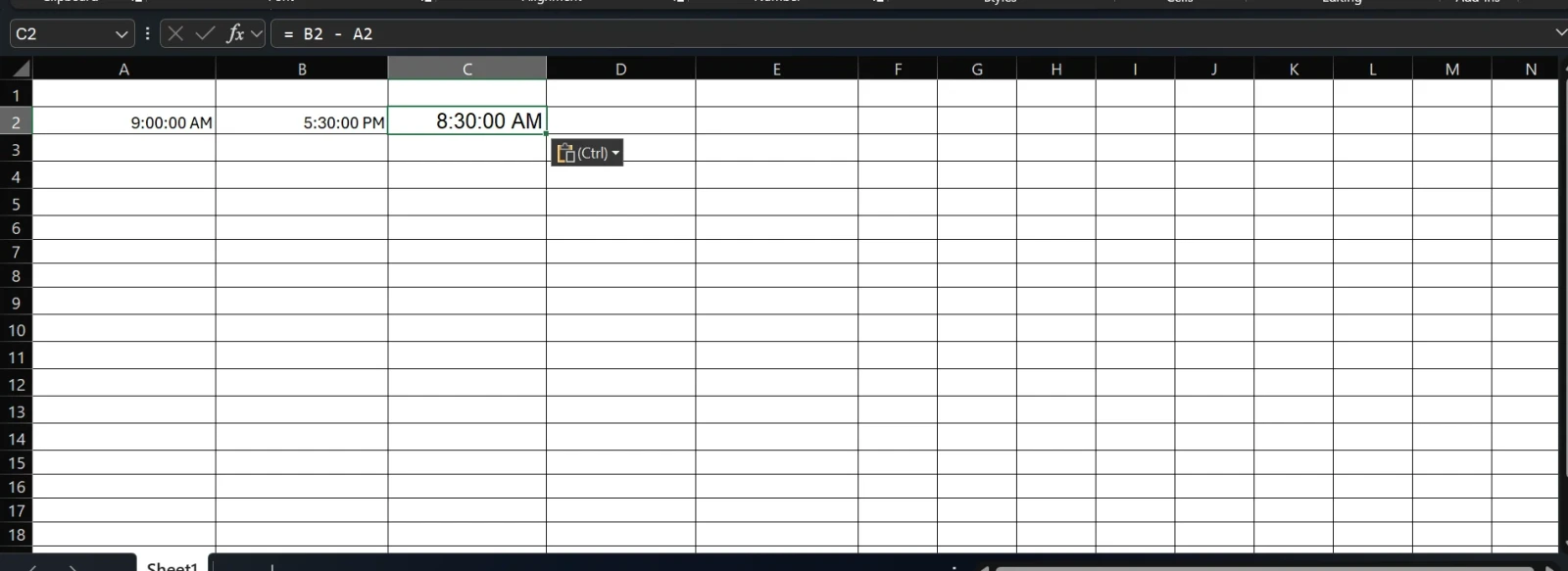
If A2 is 09:00 and B2 is 17:30, the result is 8:30 (8 hours, 30 minutes).
Important: Format the result cell as [h]:mm (not just h:mm) if the elapsed time might exceed 24 hours. To do this: right-click → Format Cells → Custom → type [h]:mm.
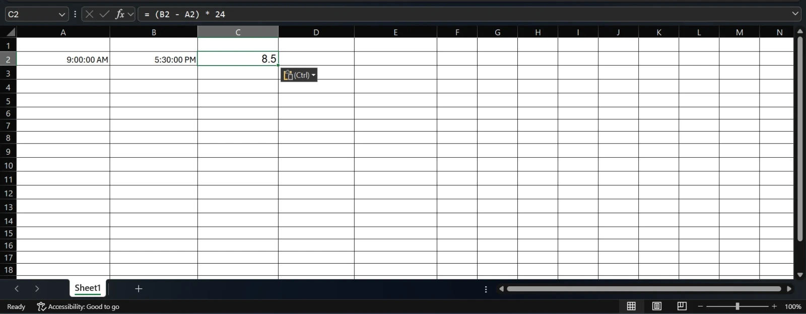
= (B2 - A2) * 24 |
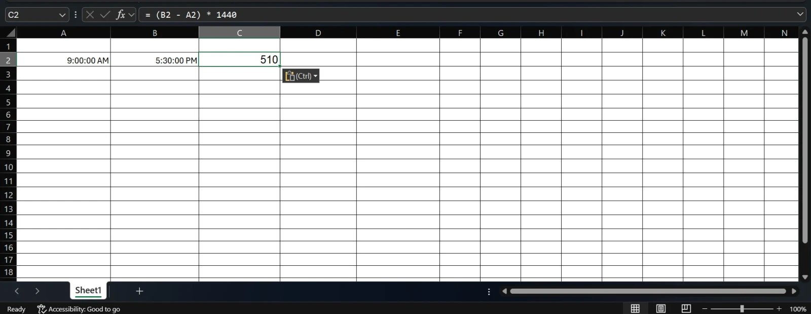
= (B2 - A2) * 1440 |
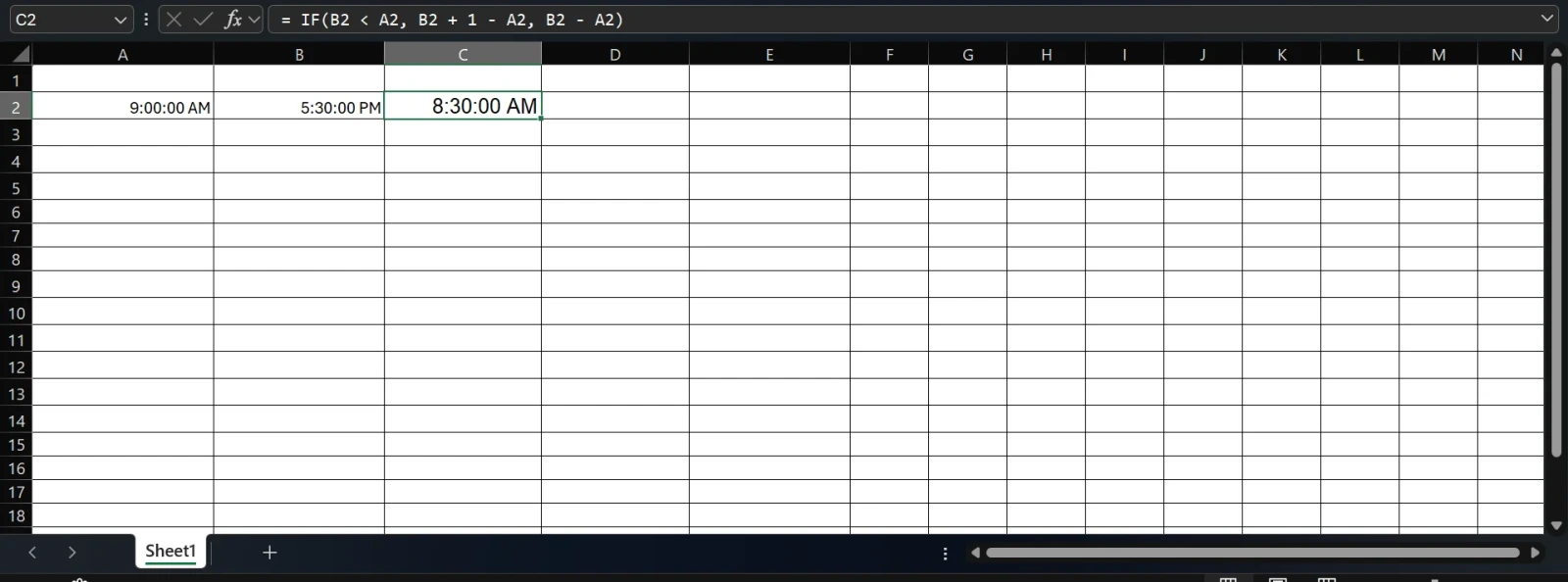
= IF(B2 < A2, B2 + 1 - A2, B2 - A2) |
This adds 1 (one full day) to the end time when the shift crosses midnight, for example, a 10 PM to 6 AM shift.
Read Also: CALCULATE Function in Power BI
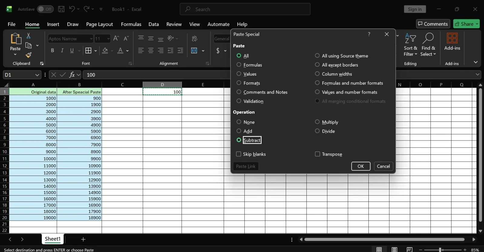
If you want to subtract a value from a range of cells permanently, without using a formula column, Paste Special is your tool.
Excel subtracts 100 from every value in the selected range and overwrites the original values. This is useful for quick bulk edits, but note that the change is permanent; the original values are replaced.
If your data is spread across worksheets, you can reference cells from other sheets directly in your subtraction formula.
Syntax:
= Sheet1!A2 - Sheet2!A2 |
Example:
= Sheet2!A2 - Sheet1!A2 |
This is powerful for building monthly comparison dashboards or financial summaries across worksheets.
Also Read: KPI in Power BI: Key Performance Indicators Dashboards
Excel follows PEMDAS strictly. If you are combining subtraction with multiplication or division in the same formula, the order matters.
| Formula | What Excel Does | Result |
|---|---|---|
= 20 - 4 * 2 |
Multiplies 4×2 first, then subtracts | 12 |
= (20 - 4) * 2 |
Subtracts first (parentheses), then multiplies | 32 |
= 100 - 50 / 5 |
Divides 50÷5 first, then subtracts | 90 |
= (100 - 50) / 5 |
Subtracts first, then divides | 10 |
Always add parentheses whenever you combine operations to make your intention explicit and avoid unexpected results.
| Scenario | Formula |
|---|---|
| Subtract two numbers | = 500 - 200 |
| Subtract two cells | = A2 - B2 |
| Subtract multiple cells | = A2 - B2 - C2 - D2 |
| Subtract a range using SUM | = A1 - SUM(A2:A10) |
| Subtract fixed value from column | = A2 - $C$1 |
| Reduce a value by a percentage | = A2 * (1 - B2) |
| Days between two dates | = B2 - A2 |
| Working days between two dates | = NETWORKDAYS(A2, B2) |
| Elapsed time (hours:minutes) | = B2 - A2 (format as [h]:mm) |
| Elapsed time in decimal hours | = (B2 - A2) * 24 |
| Cross-sheet subtraction | = Sheet2!A2 - Sheet1!A2 |
Related Article: What is Azure Virtual Machine?
Here are some fo the most common mistakes a beginner can make while performing subtraction. You just have to avoid these silly mistakes for becoming a proficient expert.
=IF(B2<A2, B2+1-A2, B2-A2) to handle overnight spans.Subtraction is just the beginning. Once you have this down, these related Excel operations are the natural next steps:
Read Also: What is POML (Prompt Orchestration Markup Language)?
Subtraction in Excel is far more versatile than most people realize. The minus sign is your core tool, but knowing how to apply it to columns, fixed values, percentages, dates, and times, along with smart techniques like absolute references and Paste Special, transforms a simple operator into a powerful analytical tool.
Whether you are building a budget tracker, calculating project timelines, analyzing sales variances, or processing time logs, the techniques in this guide cover everything you need to do the job accurately and efficiently.
No. Excel does not have a dedicated SUBTRACT function. All subtraction is done using the minus (-) operator in a formula, like =A2-B2. For subtracting a range of values, you can combine it with SUM: =A1-SUM(A2:A10).
Enter your subtraction formula in the first row (e.g., =B2-C2), then drag the fill handle down or double-click it to copy the formula through the rest of the column. Excel adjusts the row references automatically for each row.
Use an absolute cell reference: store the number in a separate cell (e.g., E1) and write =A2-$E$1. The $ signs lock E1 so it does not shift when you copy the formula down. Alternatively, use Paste Special → Subtract to apply the deduction directly to the cells without a formula.
Simply enter =B2-A2, where B2 is the later date and A2 is the earlier date. Format the result cell as a Number (not Date) to see the day count. For working days only, use =NETWORKDAYS(A2,B2).
Use =(B2-A2)*24 to get elapsed time as a decimal number of hours. To show it in h:mm format, use =B2-A2 and format the result cell as [h]:mm via Format Cells → Custom.
It means the column is too narrow to display the value, or the result is negative (which dates and times cannot display). Widen the column, and if the result is truly negative (end time is before start time), use the overnight correction formula: =IF(B2<A2, B2+1-A2, B2-A2).
Yes. Use the sheet name followed by an exclamation mark: =Sheet2!A2 - Sheet1!A2. If the sheet name contains spaces, wrap it in single quotes: ='Jan 2025'!A2 - 'Dec 2024'!A2.