Working with Excel data becomes confusing the moment you apply filters. Your totals stop making sense, numbers don’t match, and you’re left wondering what went wrong. This is exactly where the SUBTOTAL function in Excel becomes a game-changer. It lets you calculate totals that automatically adjust based on visible data, making your analysis accurate and reliable.
In this article, you’ll learn what the SUBTOTAL function is, how it works, the meaning of different function numbers, and how to use it with real examples you can try yourself. By the end, you’ll be able to handle filtered data confidently and build smarter Excel reports without errors. Let’s begin.
Read Also: How to Find Standard Deviation in Excel?
The SUBTOTAL function in Excel is a built-in function used to perform calculations like SUM, AVERAGE, COUNT, MAX, and MIN on a selected range of data. What makes it different from regular formulas is that it works intelligently with filtered data.
When you apply filters in Excel, normal functions like SUM still calculate all values, even the hidden ones. But SUBTOTAL only considers visible rows, which makes your results more accurate and meaningful. This is especially useful when working with large datasets, reports, or dashboards where you frequently filter data based on categories.
Another important feature of SUBTOTAL is that it gives you flexibility through function numbers. These numbers define what type of calculation you want to perform. For example, you can use one number for SUM and another for AVERAGE. You can also choose whether to include or ignore manually hidden rows.
In simple terms, SUBTOTAL helps you perform dynamic calculations that automatically adjust when your data view changes. Because of this, it is widely used in business analysis, financial reporting, and data management tasks where accuracy and flexibility are important.
At first, SUM seems enough. It adds numbers quickly and works well for simple data. But the moment you start filtering your dataset, SUM shows its limitation. It still includes hidden rows in the calculation, which can give you misleading results.
This is where the SUBTOTAL function in Excel becomes a better choice. It calculates only the visible data, meaning your totals automatically update when filters are applied. You don’t need to adjust formulas again and again.
Another advantage is flexibility. With SUBTOTAL, you can do more than just SUM. You can calculate AVERAGE, COUNT, MAX, and more using different function numbers, all within the same function.
It also avoids double counting. If your dataset already contains subtotals, the SUBTOTAL function ignores them, keeping your results clean and accurate.
In short, SUM is static, while SUBTOTAL is dynamic. If you are working with filtered data, reports, or dashboards, SUBTOTAL saves time, reduces errors, and gives you results you can actually trust.
Also Read: How to Subtract in Excel?
The SUBTOTAL function in Excel follows a simple and flexible structure. Once you understand the syntax, using it becomes very easy.
function_num
This defines the type of calculation you want to perform.
For example:
9 → SUM
1 → AVERAGE
2 → COUNT
109 → SUM (ignores hidden rows)
ref1
This is the main range of cells you want to calculate. Example: B2:B10
[ref2], ... (Optional)
You can add more ranges if needed. This is optional and not always required.
This calculates the SUM of values in the range C2 to C8.
Tip: The most important part of this function is the function number. It controls:
What calculation is performed
Whether hidden rows are included or ignored
The most important part of the SUBTOTAL function in Excel is the function number. This number tells Excel what calculation to perform and whether hidden rows should be included or ignored. Excel provides two sets of function numbers. The first set (1–11) includes manually hidden rows, while the second set (101–111) ignores them.
Understanding this is key because it gives you full control over how your data is calculated, especially when working with filtered reports or dashboards.
| Function | Include Hidden Rows | Ignore Hidden Rows |
| AVERAGE | 1 | 101 |
| COUNT | 2 | 102 |
| COUNTA | 3 | 103 |
| MAX | 4 | 104 |
| MIN | 5 | 105 |
| PRODUCT | 6 | 106 |
| STDEV | 7 | 107 |
| STDEVP | 8 | 108 |
| SUM | 9 | 109 |
| VAR | 10 | 110 |
| VARP | 11 | 111 |
1–11 → Includes manually hidden rows
101–111 → Ignores manually hidden rows (recommended for most cases)
For practical use, most people prefer the 100+ series because it keeps calculations clean and focused only on visible data.
Read Also: KPI in Power BI: Key Performance Indicators Dashboards
Now that you understand how the SUBTOTAL function works, let’s apply it in real scenarios.
Goal: To calculate the total revenue that automatically updates when filters are applied.
FORMULA:
=SUBTOTAL(109, C2:C7)
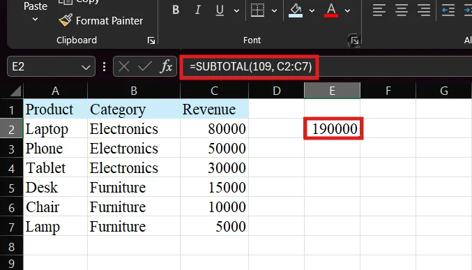
In this example, I have used function number 109 that means SUM while ignoring hidden rows. Initially, the formula calculates the total revenue of all products. But the real power appears when you apply a filter. For example, if you filter only Electronics, the formula will automatically update and show the total revenue of just those visible rows.
Unlike the normal SUM function, this formula does not include hidden or filtered-out data. This makes it extremely useful for reports where you frequently change views using filters.
Goal: To count how many products are currently visible after applying filters.
FORMULA: =SUBTOTAL(103, A2:A7)
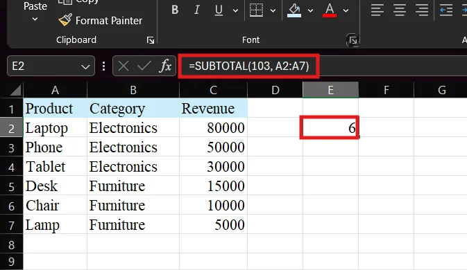
In this example, I used function number 103, which represents COUNTA and ignores hidden rows. This formula counts all non-empty cells in the Product column, but only for visible rows. So, if you apply a filter (for example, showing only Furniture), the count will automatically adjust to show only the visible products.
This is especially helpful when you want to track how many records meet certain conditions without manually counting or updating formulas.
Read Also: How to Remove Blank Rows in Excel?
Goal: To calculate the average revenue based only on visible data.
FORMULA:
=SUBTOTAL(101, C2:C7)
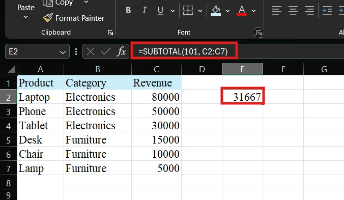
In this example, I used function number 101, which calculates the AVERAGE while ignoring hidden rows. When no filter is applied, it calculates the average of all revenue values. But once you filter the data, the formula automatically updates and calculates the average only for the visible rows.
This is very useful in analysis scenarios where you want insights based on a selected category instead of the entire dataset.
In this section, my goal is to calculate total revenue that updates automatically when filters are applied by using the SUBTOTAL function. Let’s begin.
FORMULA: =SUBTOTAL(109, C2:C8)
Now, you just need to follow these simple steps to see how the SUBTOTAL function works with filters in real time.
Paste the dataset into Excel properly with headers (Product, Category, Revenue). Make sure your data is clean and aligned in columns.
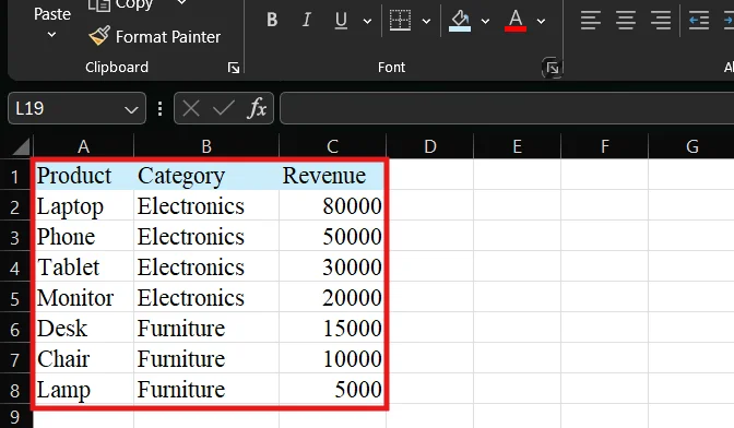
Now, you need to select the entire dataset
Next, go to Data and then apply Filter
You will see dropdown arrows appear in the header row
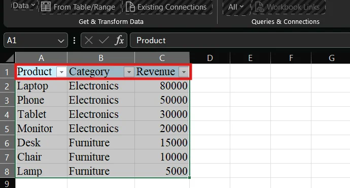
Now, go in any empty cell (for example, C10) and enter this formula: =SUBTOTAL(109, C2:C8). At this point, it will show you the total revenue of all products.
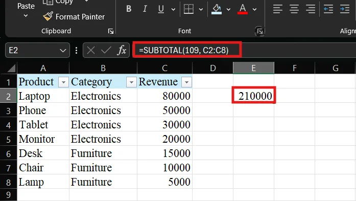
First, go and click the filter dropdown in the Category column.
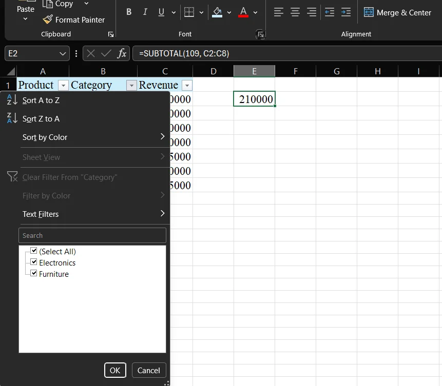
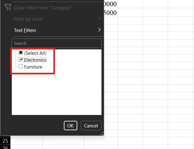
Then here, you need to select only Electronics.
Now, the worksheet displays only Electronics records, and the subtotal updates automatically to 180,000.
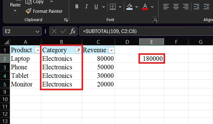
Explanation: When you applied the SUBTOTAL formula, Excel calculated the total revenue using function number 109, which means SUM while ignoring hidden rows.
Initially, all rows were visible, so the formula returned the total of the entire dataset. But once you applied a filter and selected only Electronics, Excel automatically hid the other rows.
The SUBTOTAL function responded to this change and recalculated the total based only on the visible rows. This is what makes it different from the normal SUM function, which would still include all values.
In simple terms, the formula adjusts itself based on what you are viewing. This makes it extremely useful for real-time analysis, reports, and dashboards where data is constantly filtered.
Read Also: How to Use HLOOKUP Function?
At first glance, the two sets of SUBTOTAL function numbers might look confusing. But the difference is actually simple and very important in real use.
The numbers 1–11 include manually hidden rows in the calculation. This means if you hide rows using “Hide” in Excel, those values are still counted. On the other hand, 101–111 ignores manually hidden rows, so only visible data is used.
Now here’s the key point. Both sets automatically ignore filtered rows. So even if you use 9 or 109, filtered-out data will not be included. The real difference shows up only when rows are hidden manually.
When you want to include hidden rows
If rows are hidden temporarily but still important for your total, this option ensures nothing is missed.
When data visibility is not affecting calculations
For static reports where hiding rows is just for better viewing, not analysis, using 1–11 works fine.
When you want accurate visible-only calculations
This is the most common case. If you are analyzing filtered or cleaned data, you want only visible rows included.
When building dashboards or reports
Dashboards often involve hiding unnecessary data. Using 101–111 ensures your results stay clean and relevant.
When avoiding calculation errors
Ignoring hidden rows prevents accidental inclusion of unwanted data, which improves accuracy.
Both SUM and SUBTOTAL are used to calculate totals in Excel, but they behave very differently when your data changes. While SUM is simple and works well for basic calculations, it does not adjust when you filter or hide data. SUBTOTAL, on the other hand, is designed for dynamic datasets and updates results based on what is visible. This makes it much more useful for real-world analysis, reports, and dashboards.
| Feature | SUM Function | SUBTOTAL Function |
| Basic calculation | Adds numbers | Adds numbers (and more) |
| Works with filters | No | Yes |
| Ignores filtered rows | No | Yes |
| Ignores manually hidden rows | No | Yes (with 101–111) |
| Supports multiple operations | No (only SUM) | Yes (SUM, AVERAGE, COUNT, etc.) |
| Dynamic updates | No | Yes |
| Avoids double counting | No | Yes |
Also Read: XLOOKUP() vs. VLOOKUP()
Both SUBTOTAL and AGGREGATE are powerful Excel functions used for calculations on datasets, especially when working with filtered or hidden data. While SUBTOTAL is simple and widely used, AGGREGATE is more advanced and gives you extra control, especially when dealing with errors and complex scenarios.
| Feature | SUBTOTAL Function | AGGREGATE Function |
| Ease of use | Very simple | Slightly complex |
| Functions supported | 11 functions | 19 functions |
| Works with filters | Yes | Yes |
| Ignores hidden rows | Yes (with 101–111) | Yes |
| Ignores errors (like #DIV/0!) | No | Yes |
| Ignores nested subtotals | Yes | Yes |
| Supports arrays | No | Yes |
| Best for | Basic reporting | Advanced analysis |
Even though the SUBTOTAL function in Excel is simple to use, small mistakes can lead to incorrect results. Most errors happen because of wrong function numbers, incorrect ranges, or misunderstanding how hidden and filtered rows work. The good part is that these issues are easy to fix once you know what to check.
One of the most common mistakes is selecting the wrong function number. For example, using 9 instead of 109 can include hidden rows when you actually want to ignore them.
Fix: Always double-check whether you need to include or ignore hidden rows. In most cases, use the 101–111 series for accurate results.
Many users expect SUBTOTAL to behave differently without applying filters. But if no filter is applied, the result will look the same as a normal formula.
Fix: Apply filters to your dataset to see the dynamic behavior of SUBTOTAL.
If your range is wrong or incomplete, your result will also be incorrect. For example, selecting only part of the data can give a lower total.
Fix: Always verify that your range (like C2:C8) covers the full dataset.
SUBTOTAL treats filtered and manually hidden rows differently. Many users assume both behave the same way.
Fix: Remember:
Filtered rows are always ignored
Hidden rows are ignored only with 101–111
Sometimes users accidentally include column headers in the formula range, which can affect functions like COUNT or AVERAGE.
Fix: Start your range from actual data rows (e.g., C2, not C1).
If your data already contains SUBTOTAL formulas, Excel automatically ignores them to prevent double counting. This can confuse users who expect those values to be included.
Fix: Understand that this is intentional behavior. If needed, adjust your structure or use a different approach.
Read Also: How to Separate Names in Excel?
The SUBTOTAL function in Excel is best used when your data is not static. If you are simply adding numbers in a fixed dataset, a normal SUM formula works fine. But the moment your data involves filtering, hiding, or frequent changes, SUBTOTAL becomes the better choice.
It is mainly used in situations where you want your calculations to adjust automatically based on what is visible on the screen.
If you apply filters to your dataset, SUBTOTAL ensures that only visible rows are calculated. This makes your totals accurate and relevant without needing to change the formula again and again.
In reports, you often hide or filter data to focus on specific insights. SUBTOTAL helps maintain dynamic totals that update instantly as the data view changes. This is very useful in business and financial reports.
Instead of using separate formulas like SUM, AVERAGE, or COUNT, you can use SUBTOTAL with different function numbers. This keeps your formulas simple and consistent.
If your dataset already includes subtotals, SUBTOTAL automatically ignores them. This prevents errors and keeps your final result accurate.
In large Excel sheets, manually adjusting formulas can be time-consuming. SUBTOTAL saves time by automatically adapting to filters and hidden data.
The SUBTOTAL function in Excel is one of the most useful tools for working with filtered and dynamic data. Unlike regular formulas, it updates automatically based on visible rows, making your calculations more accurate and reliable.
By understanding function numbers and how filtering affects results, you can use SUBTOTAL for real-world tasks like reports, dashboards, and data analysis. Whether you are calculating totals, averages, or counts, this function helps you save time and avoid common errors.
Once you start using SUBTOTAL in your workflow, managing large datasets becomes much easier and more efficient.
Explore Other Microsoft-Related Articles:
FAQs
SUBTOTAL performs calculations like SUM, AVERAGE, and COUNT while considering only visible data in a filtered dataset.
9 includes hidden rows, while 109 ignores hidden rows and calculates only visible data.
Yes, SUBTOTAL automatically ignores filtered rows in all cases.
Yes, SUBTOTAL can replace SUM, especially when working with filtered or dynamic datasets.